R is a free software environment for statistical computing and graphics that provides a programming language and built-in libraries of mathematics operations for statistics, data analysis, machine learning and much more. Many domain experts and researchers use the R platform and contribute R software, resulting in a large ecosystem of free software packages available through CRAN (the Comprehensive R Archive Network).
However, R, like many other high-level languages, is not performance competitive out of the box with lower-level languages like C++, especially for highly data- and computation-intensive applications. R programs tend to process large amounts of data, and often have significant independent data and task parallelism. Therefore, R applications stand to benefit from GPU acceleration. This way, R users can benefit from R’s high-level, user-friendly interface while achieving high performance.
In this article, I will introduce the computation model of R with GPU acceleration, focusing on three topics:
- accelerating R computations using CUDA libraries;
- calling your own parallel algorithms written in CUDA C/C++ or CUDA Fortran from R; and
- profiling GPU-accelerated R applications using the CUDA Profiler.
The GPU-Accelerated R Software Stack
Figure 1 shows that there are two ways to apply the computational power of GPUs in R:
- use R GPU packages from CRAN; or
- access the GPU through CUDA libraries and/or CUDA-accelerated programming languages, including C, C++ and Fortran.
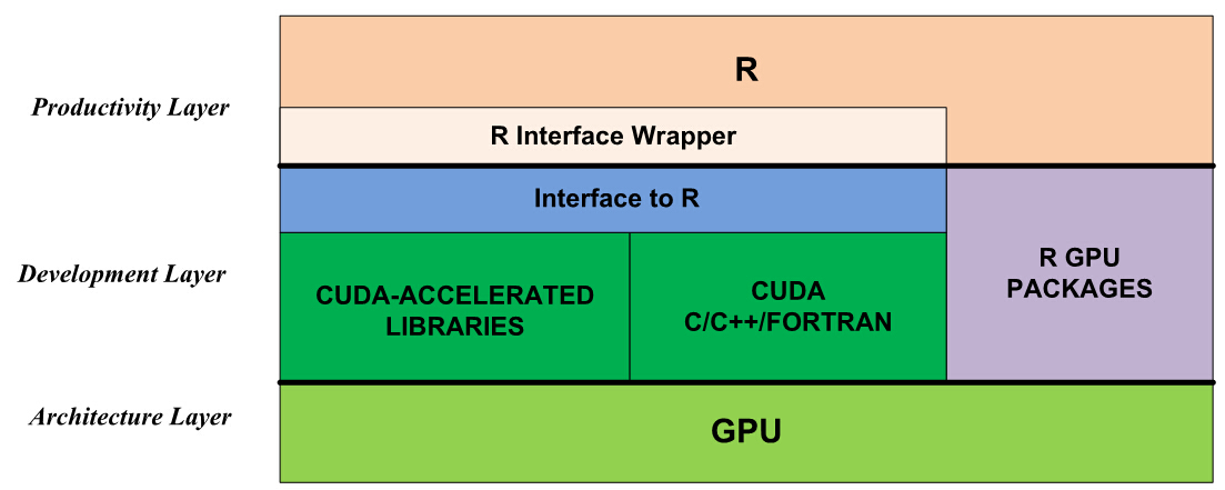
The first approach is to use existing GPU-accelerated R packages listed under High-Performance and Parallel Computing with R on the CRAN site. Examples include gputools and cudaBayesreg. These packages are very easy to install and use. On the other hand, the number of GPU packages is currently limited, quality varies, and only a few domains are covered. This will improve with time.
The second approach is to use the GPU through CUDA directly. While the CUDA ecosystem provides many ways to accelerate applications, R cannot directly call CUDA libraries or launch CUDA kernel functions. To solve this problem, we need to build an interface to bridge R and CUDA the development layer of Figure 1 shows. For productivity, we should also encapsulate these interface functions in the R environment, so that the technical changes between the CPU and GPU are transparent to the R user. (Note that this wrapper is optional; the user can also call the R interface function directly from R.)
Accelerate R using CUDA Libraries
As you know, there are many GPU-accelerated libraries (from NVIDIA as well as third-party and open-source libraries) that provide excellent usability, portability and performance. Using GPU-accelerated libraries reduces development effort and risk, while providing support for many NVIDIA GPU devices with high performance. Thus, CUDA libraries are a quick way to speed up applications, without requiring the R user to understand GPU programming.
I will show you step-by-step how to use CUDA libraries in R on the Linux platform. My example for this post uses cuFFT (version 6.5), but it is easy to use other libraries in your application with the same development flow.
The FFT Target Function
In this case, we want to implement an accelerated version of R’s built-in 1D FFT. Here is the description of the R FFT.
Fast Discrete Fourier Transform
        Description
         Performs the Fast Fourier Transform of an array.
        Usage
         fft(z, inverse = FALSE)
        Arguments
        z : a real or complex array containing the values to be
         transformed.
        inverse : if TRUE, the unnormalized inverse transform is computed
         (the inverse has a + in the exponent of e, but here, we
         do not divide by 1/length(x)).
Writing an Interface Function
First of all, we need to implement the interface code between R and C. The functions we write with (CUDA) C need to satisfy several properties.
- C functions called by R must have a
voidreturn type, and should return results via the function arguments. - R passes all arguments to C functions by reference (using pointers), so we must dereference the pointers in C (even scalar input arguments).
- Each file containing C functions to be called from R should include R.h and the header files for any CUDA libraries used by the function.
The following code defines our interface function.
#include <r.h>
#include <cufft.h>
/* This function is written for R to compute 1D FFT.
   n - [IN] the number of complex we want to compute
   inverse - [IN] set to 1 if use inverse mode
   h_idata_re - [IN] input data from host (R, real part)
   h_idata_im - [IN] input data from host (R, imaginary part)
   h_odata_re - [OUT] results (real) allocated by caller
   h_odata_im - [OUT] results (imaginary) allocated by caller
*/
extern "C"
void cufft(int *n, int *inverse, double *h_idata_re,
           double *h_idata_im, double *h_odata_re, double *h_odata_im)
{
  cufftHandle plan;
  cufftDoubleComplex *d_data, *h_data;
  cudaMalloc((void**)&d_data, sizeof(cufftDoubleComplex)*(*n));
  h_data = (cufftDoubleComplex *) malloc(sizeof(cufftDoubleComplex) * (*n));

  // Convert data to cufftDoubleComplex type
  for(int i=0; i< *n; i++) {
    h_data[i].x = h_idata_re[i];
    h_data[i].y = h_idata_im[i];
  }

  cudaMemcpy(d_data, h_data, sizeof(cufftDoubleComplex) * (*n),
             cudaMemcpyHostToDevice);
  // Use the CUFFT plan to transform the signal in place.
  cufftPlan1d(&plan, *n, CUFFT_Z2Z, 1);
  if (!*inverse ) {
    cufftExecZ2Z(plan, d_data, d_data, CUFFT_FORWARD);
  } else {
    cufftExecZ2Z(plan, d_data, d_data, CUFFT_INVERSE);
  }

  cudaMemcpy(h_data, d_data, sizeof(cufftDoubleComplex) * (*n),
  cudaMemcpyDeviceToHost);
  // split cufftDoubleComplex to double array
  for(int i=0; i<*n; i++) {
    h_odata_re[i] = h_data[i].x;
    h_odata_im[i] = h_data[i].y;
  }

  // Destroy the CUFFT plan and free memory.
  cufftDestroy(plan);
  cudaFree(d_data);
  free(h_data);
}
This file includes two header files, “R.h” and “cufft.h”. We write a C function called cufft, and declare it extern "C" so that we can call it from R. The first four arguments are input arguments and the last two are output arguments which we use to pass computation results back to R. Because of data type differences between R and cufft, we pass the real and imaginary parts separately and combine them together to fill the array of cufftComplex structures. We then copy the complex array to the device.
We call cufftExecC2C() to do a 1D FFT, choosing CUFFT_FORWARD or CUFFT_INVERSE depending on the value of the inverse argument. Then we copy the result back from device to host and assign the result to the output arguments h_odata_re and h_odata_im . Finally, we destroy temporary objects and free the allocated memory.
Compile and Link a Shared Object
Now that we’ve written our interface function, we need to compile and link it into a shared object file (.so). We compile the source code to an object file with the optimization option -O3, and then link the object file with libcufft and libR into a shared object file. (NOTE: if you don’t find libR.so in your R lib directory, you can rebuild the R package with ‘–enable-R-shlib’ configuration.)
nvcc -O3 -arch=sm_35 -G -I/usr/local/cuda/r65/include
         -I/home/patricz/tools/R-3.0.2/include/
         -L/home/patricz/tools/R/lib64/R/lib -lR
         -L/usr/local/cuda/r65/lib64 -lcufft
         --shared -Xcompiler -fPIC -o cufft.so cufft-R.cu
Load shared object in wrapper
Now that we have our interface function in a shared object, we just need to load cufft-R.so and call our new API. We load external C code in R using the function dyn.load(), and we can use the is.loaded() function to check if our API is available in the R environment.
Once our function is loaded, we call it using R’s .C() function, passing our function name (cufft) as the first argument followed by the arguments for cufft(). More importantly, we must tell R of the explicit type of each argument, using as.<type>(). But it’s tedious and error-prone to call .C() every time we need to use our custom function. So the best practice is to write an interface wrapper in R. As the following code shows, the wrapper loads our shared object, calls cufft() via .C(), and then converts the output into the complex data type. Now, we can use this wrapper routine in the same way as R’s built-in FFT.
cufft1D <- function(x, inverse=FALSE)
{
  if(!is.loaded("cufft")) {
    dyn.load("cufft.so")
  }
  n <- length(x)
  rst <- .C("cufft",
  as.integer(n),
  as.integer(inverse),
  as.double(Re(z)),
  as.double(Im(z)),
  re=double(length=n),
  im=double(length=n))
  rst <- complex(real = rst[["re"]], imaginary = rst[["im"]])
  return(rst)
}
Execution and Testing
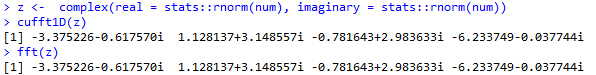
So far, so good! Let’s try our new cufft function in R. You can see that we can now use the GPU-accelerated FFT as easily as R’s built-in FFT, and that both versions compute the same result.
> source("wrap.R")
> num <- 4
> z <- complex(real = stats::rnorm(num), imaginary = stats::rnorm(num))
> cpu <- fft(z)
[1] 1.140821-1.352756i -3.782445-5.243686i 1.315927+1.712350i -0.249490+1.470354i
> gpu <- cufft1D(z)
[1] 1.140821-1.352756i -3.782445-5.243686i 1.315927+1.712350i -0.249490+1.470354i
> cpu <- fft(z, inverse=T)
[1] 1.140821-1.352756i -0.249490+1.470354i 1.315927+1.712350i -3.782445-5.243686i
> gpu <- cufft1D(z, inverse=T)
[1] 1.140821-1.352756i -0.249490+1.470354i 1.315927+1.712350i -3.782445-5.243686i
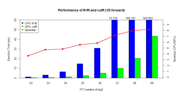
Now, let’s see what performance we can gain from GPU acceleration. We tested on an 8-core Intel® Xeon® CPU (E5-2609 @ 2.40GHz / 64GB RAM) and NVIDIA GPU (Tesla K20Xm with 6GB device memory). As shown in Figure 3, cufft provides 3x-8x speedup compared with R’s built-in FFT.
Accelerate R using CUDA C/C++/Fortran
When R GPU packages and CUDA libraries don’t offer the functionality you need, you can write custom GPU-accelerated code using CUDA. The process is very similar to our previous example of a CUDA library call; the only difference is that you need to write a parallel function yourself.
In the following example code, we implement vector addition on the GPU and call it from our interface function gvectorAdd. In practice you can implement any algorithm and call it from an interface function as in this example. The remaining steps (building a shared object and writing an R wrapper) are similar to my previous example.
extern "C" void gvectorAdd(double *A, double *B, double *C, int *n);

__global__ void
vectorAdd(const double *A, const double *B, double *C, int numElements)
{
  int i = blockDim.x * blockIdx.x + threadIdx.x;
  if(i < numElements)
  {
    C[i] = A[i] + B[i];
  }
}

void gvectorAdd(double *A, double *B, double *C, int *n)
{
  // Device Memory
  double *d_A, *d_B, *d_C;
  // Define the execution configuration
  dim3 blockSize(256,1,1);
  dim3 gridSize(1,1,1);
  gridSize.x = (*n + blockSize.x - 1) / blockSize.x;
  // Allocate output array
  cudaMalloc((void**)&d_A, *n * sizeof(double));
  cudaMalloc((void**)&d_B, *n * sizeof(double));
  cudaMalloc((void**)&d_C, *n * sizeof(double));
  // copy data to device
  cudaMemcpy(d_A, A, *n * sizeof(double), cudaMemcpyHostToDevice);
  cudaMemcpy(d_B, B, *n * sizeof(double), cudaMemcpyHostToDevice);
  // GPU vector add
  vectorAdd<<<gridSize,blockSize>>>(d_A, d_B, d_C, *n);
  // Copy output
  cudaMemcpy(C, d_C, *n * sizeof(double), cudaMemcpyDeviceToHost);
  cudaFree(d_A);
  cudaFree(d_B);
  cudaFree(d_C);
}
CUDA Performance Profiling
When developing GPU code or using GPU packages in R, you may encounter functional and performance problems. To solve these problems efficiently, you can use CUDA developer tools such as cuda-gdb, Nsight and the NVIDIA Visual Profiler or nvprof. For this example, I will show you how to profile our cuFFT example above using nvprof, the command line profiler included with the CUDA Toolkit (check out the post about how to use nvprof to profile any CUDA program). My testing environment is R 3.0.2 on a 12-core Intel® Xeon® CPU (E5645 @ 2.40GHz and 24G RAM) combined with an NVIDIA Tesla GPU (K20Xm with 6GB device memory).
There are two approaches to launching nvprof with R.
- Use
nvprofas a wrapper to launch R by typing nvprof R, then run the GPU solver and exit, or usenvprofto launch R with a batch script:nvprof R CMD BATCH script.R - Launch
nvprof --profile-all-processesin a separated console. R executes the GPU solver and exits as normal, andnvprofin another console captures the GPU behavior and prints the profile.
Here is the nvprof output for our FFT wrapper function, for a signal of 2^26 elements:
==18067== Profiling application: /home/patricz/tools/R/lib64/R/bin/exec/R
==18067== Profiling result:
 Time(%) Time Calls Avg Min Max Name
  55.41% 277.50ms 1 277.50ms 277.50ms 277.50ms [CUDA memcpy HtoD]
  39.30% 196.82ms 1 196.82ms 196.82ms 196.82ms [CUDA memcpy DtoH]
  1.35% 6.7531ms 1 6.7531ms 6.7531ms 6.7531ms void spRadix0128B::kernel1Mem(Complex*, Complex const *, unsigned int, unsigned int, unsigned int, divisor_t, Complex const *, Complex const *, coordDivisors_t, Coord, Coord, unsigned int, unsigned int, float, int, int)
  1.34% 6.7084ms 1 6.7084ms 6.7084ms 6.7084ms void spRadix0032B::kernel1Mem(Complex*, Complex const *, unsigned int, unsigned int, unsigned int, divisor_t, Complex const *, Complex const *, coordDivisors_t, Coord, Coord, unsigned int, unsigned int, float, int, int)
  1.30% 6.5350ms 1 6.5350ms 6.5350ms 6.5350ms void spRadix0128C::kernel1Mem(Complex*, Complex const *, unsigned int, unsigned int, unsigned int, divisor_t, Complex const *, Complex const *, coordDivisors_t, Coord, Coord, unsigned int, unsigned int, float, int, int)
  1.30% 6.4979ms 1 6.4979ms 6.4979ms 6.4979ms void spRadix0128B::kernel3Mem(Complex*, Complex const *, unsigned int, unsigned int, divisor_t, coordDivisors_t, Coord, unsigned int)
==14905== API calls:
Time(%) Time Calls Avg Min Max Name
 52.35% 502.32ms 2 251.16ms 223.84ms 278.49ms cudaMemcpy
 24.08% 231.04ms 3 77.012ms 491.74us 229.92ms cudaFree
 23.02% 220.89ms 2 110.44ms 580.53us 220.30ms cudaMalloc
 0.41% 3.9122ms 664 5.8910us 278ns 232.60us cuDeviceGetAttribute
 0.07% 625.78us 8 78.222us 67.720us 97.719us cuDeviceTotalMem
 0.05% 483.86us 8 60.482us 50.428us 106.37us cuDeviceGetName
 0.01% 81.052us 4 20.263us 13.612us 36.908us cudaLaunch
 0.01% 79.330us 1 79.330us 79.330us 79.330us cudaGetDeviceProperties
 0.00% 24.473us 56 437ns 300ns 1.0670us cudaSetupArgument
 0.00% 20.558us 7 2.9360us 538ns 9.2310us cudaGetDevice
 0.00% 14.040us 4 3.5100us 2.0570us 7.1580us cudaFuncSetCacheConfig
 0.00% 7.4470us 1 7.4470us 7.4470us 7.4470us cudaDeviceSynchronize
 0.00% 4.9390us 12 411ns 283ns 597ns cuDeviceGet
 0.00% 3.7660us 3 1.2550us 417ns 2.5800us cuDeviceGetCount
 0.00% 3.2650us 4 816ns 568ns 1.4930us cudaConfigureCall
 0.00% 2.6450us 4 661ns 314ns 1.3870us cudaPeekAtLastError
 0.00% 1.9140us 4 478ns 402ns 548ns cudaGetLastError
 0.00% 1.1380us 1 1.1380us 1.1380us 1.1380us cuDriverGetVersion
 0.00% 1.1310us 1 1.1310us 1.1310us 1.1310us cuInit
Summary
In this post, I introduced the R computation model with GPU acceleration and showed how to use the CUDA ecosystem to accelerate your R applications, and how to profile GPU performance within R.
Try CUDA with your R applications now, and have fun!
Appendix:
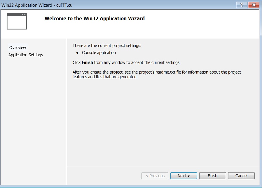
Build R Applications with CUDA by Visual Studio on Windows
- Download and install Visual Studio 2013
- Download and install CUDA toolkit
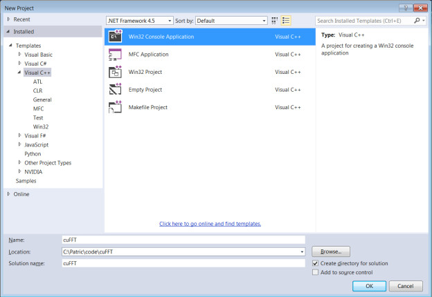
- Open VS2013, and create ‘New Project’ then you will see NVIDIA/CUDA item.
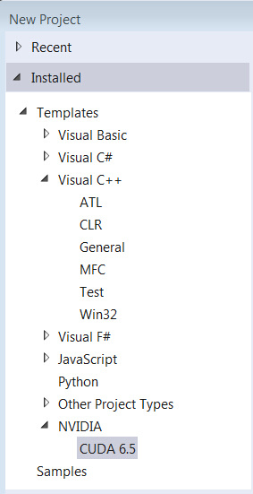
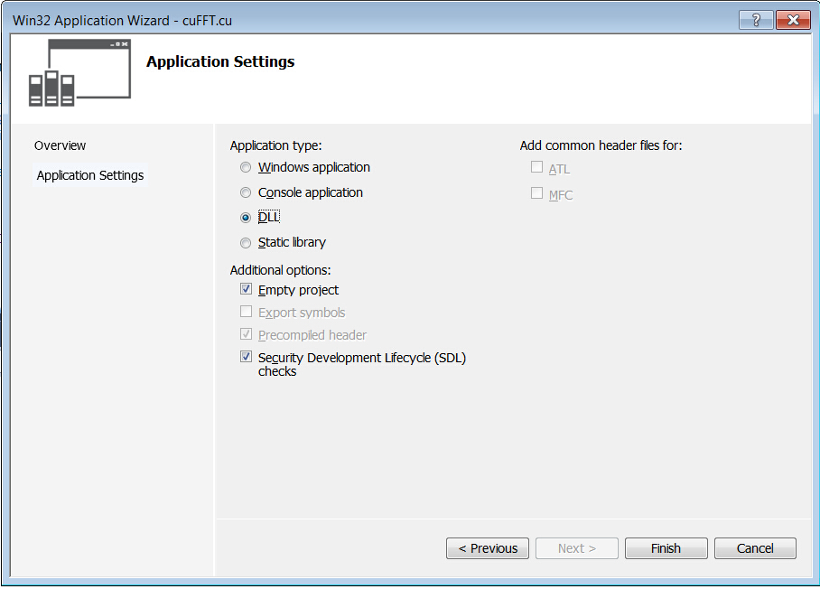
- Select ‘Visual C++’ → ‘Win32 Console Application’
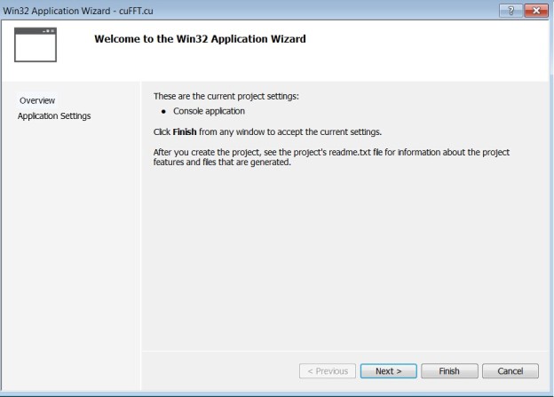
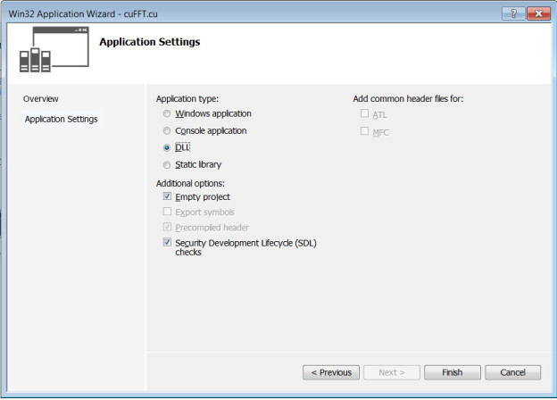
- Select ‘DLL’ for Application type to create a ‘Empty project’ in Wizard platform
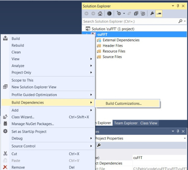
- Changes Project type to CUDA
→’Solution Explorer’
→Right click project name
→’Build Dependencies’
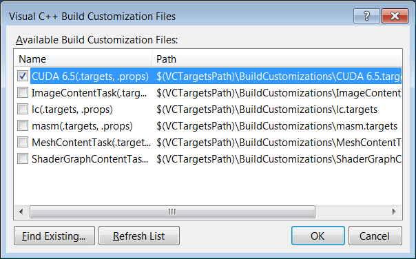
→’Build Customizations…’
→’CUDA 6.5′
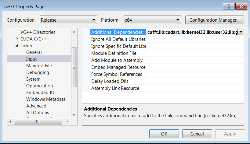
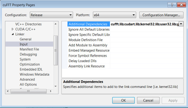
- Add CUDA and CUDA-accelerated libraries into Visual Studio project properties.
→’Solution Explorer’
→Right click project name
→’Properties’
→’Linker’
→’Input’
→’Additional Dependencies’
→Add “cufft.lib” and “cudart.lib”
Note: if you encountered the error “LNK2001: unresolved external symbol cudaXXX”, please check if you added all necessary CUDA libraries to the project properties.
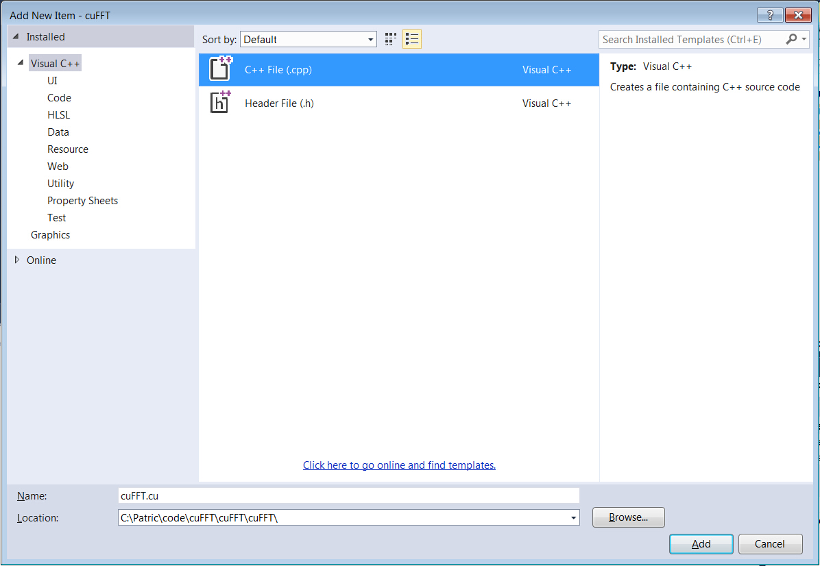
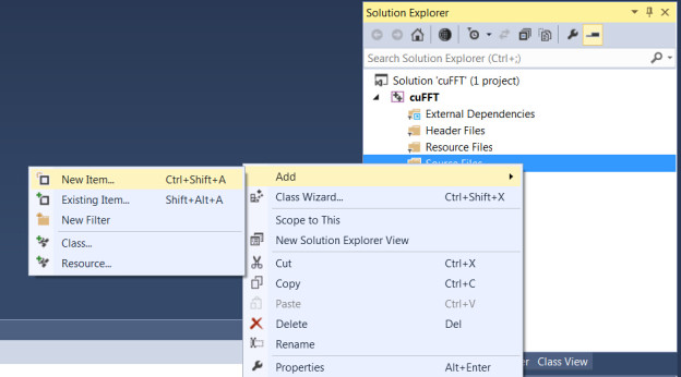
- Add a CUDA source code file with .cu suffix
→’Solution Explorer’
→’Source Files’
→’Add’
→’New Item’
→’C++ File(.cpp)’
→Type “cuFFt.cu”

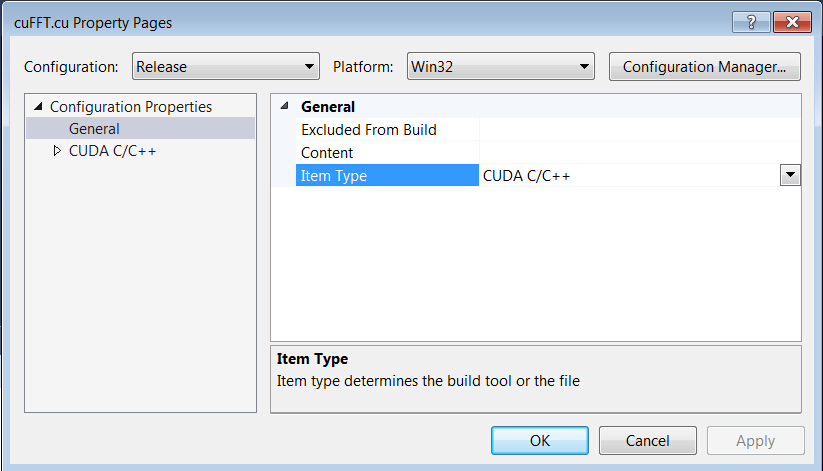
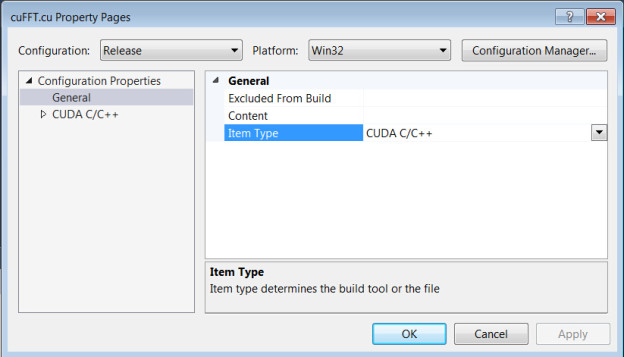
Check the ‘Item type’ of cuFFT.cu by right-clicking its filename (cuFFT.cu) and selecting ‘Properties’.
Make sure the type is set to ‘CUDA C/C++’.
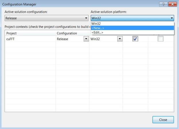
- Change to 64-bit if you are working on a 64-bit platform.
→’Build’
→’Configuration Manager’
→’Active solution platform:’
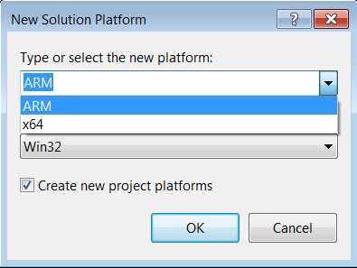
→’New’
→select ‘x64’
Note: if you encounter the error “LoadLibrary failure: %1 is not a valid Win32 application.” when you load a DLL in R, you should check if you built the DLL with R for the same platform (32- or 64-bit).
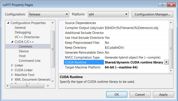
- Select 64-bit CUDA and build options for shared runtime
→‘Solution Explorer’
→Right click project name
→’Properties’
→’CUDA C/C++’
→’Common’Select :
‘Shared/dynamic CDUA runtime library’ in ‘CUDA Runtime’
’64-bit (–machine 64)’ in ‘Target Machine Platform’
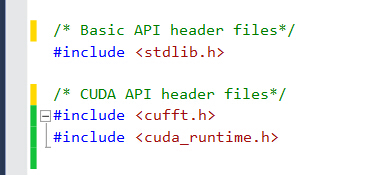
- Copy your CUDA code into this file, and add the necessary header files for CUDA.

Declare routines which need to be called from R with
extern “C” __declspec(dllexport)

- Build the Project to produce cuFFT.dll

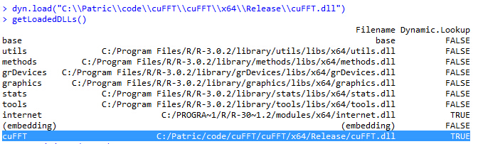
- Load cuFFT.dll in R and check the DLL path.
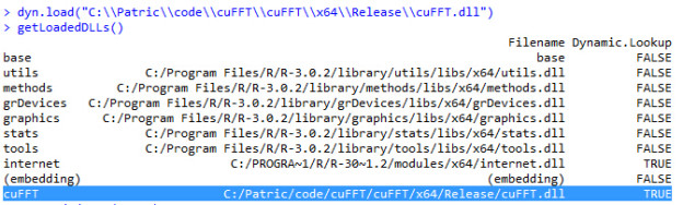
- Run cuFFT in R on Windows