Graph analysis is a fundamental tool for domains as diverse as social networks, computational biology, and machine learning. Real-world applications of graph algorithms involve tremendously large networks that cannot be inspected manually. Betweenness Centrality (BC) is a popular analytic that determines vertex influence in a graph. It has many practical use cases, including finding the best locations for stores within cities, power grid contingency analysis, and community detection. Unfortunately, the fastest known algorithm for computing betweenness centrality has 


This post describes how we used CUDA and NVIDIA GPUs to accelerate the BC computation, and how choosing efficient parallelization strategies results in an average speedup of 2.7x, and more than 10x speedup for road networks and meshes versus a naïve edge-parallel strategy.
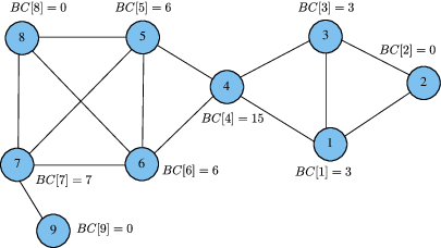
Betweenness Centrality determines the importance of vertices in a network by measuring the ratio of shortest paths passing through a particular vertex to the total number of shortest paths between all pairs of vertices. Intuitively, this ratio determines how well a vertex connects pairs of vertices in the network. Formally, the Betweenness Centrality of a vertex 
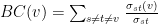
where 


Algorithms
Naïve implementations of Betweenness Centrality solve the all-pairs shortest paths problem using the 

This definition splits the calculation of BC scores into two steps:
- Find the number of shortest paths between each pair of vertices
- Sum the dependencies for each vertex
We can redefine the calculation of BC scores in terms of dependencies as follows:
Sparse Graph Representation on the GPU
The most intuitive way to store a graph in memory is as an adjacency matrix. Element 


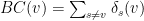
The alternative to the adjacency matrix that has been commonly used for graph applications on the GPU is the Compressed Sparse Row (CSR) format. This representation consists of two arrays: column indices and row offsets. The column indices array is a concatenation of each vertex’s adjacency list into an array of 
u starts at C[R[u]] and ends at C[R[u+1]-1] (inclusively).
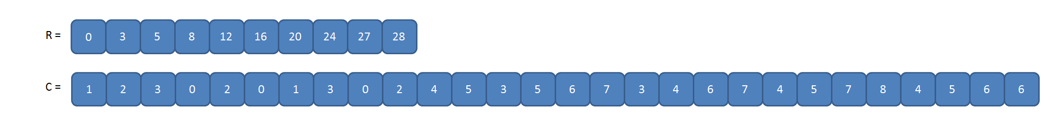
Another common alternative is the Cooperative (COO) format. This representation is essentially a list of edges. Two arrays of length C, is the same for both CSR and COO formats.
Parallelization of Betweenness Centrality in CUDA
Now that we have enough background on how to calculate Betweenness Centrality, lets discuss how we can implement it efficiently in CUDA. Since the graph traversal and shortest path accumulations of each root are independent, we can process all roots in parallel. We take advantage of this coarse-grained parallelism by assigning roots to each Streaming Multiprocessor (SM) of the GPU. Additionally, we can leverage fine-grained parallelism by having threads process the shortest path calculations and dependency accumulations cooperatively by executing level-synchronous breadth-first searches. Threads explore the neighbors of the source vertex and then explore the neighbors of those vertices and so on until there are no remaining vertices to explore. We call each set of inspected neighbors as a vertex frontier and we call the set of outgoing edges from a vertex frontier an edge frontier.
Equivalently, each CUDA thread block processes its own set of roots and the threads within the block traverse the graph cooperatively, starting at the roots assigned to their block. It turns out that the way we handle this fine-grained parallelism is the dominating performance factor, so that is the scope of optimization for this post.
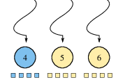
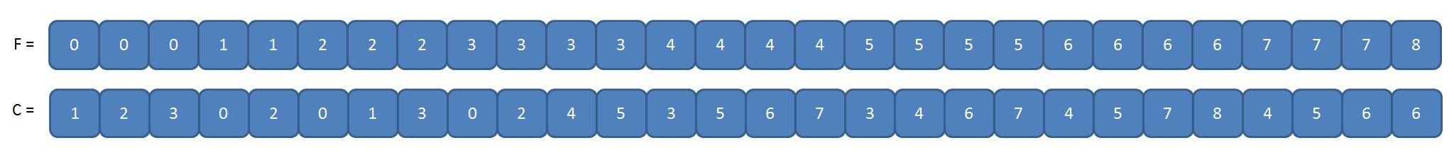
Figure 4 illustrates three methods of distributing threads to units of work, using the same example graph from Figure 1. Consider a Breadth-First Search (BFS) that expands from vertex 4. During the second iteration of the search, vertices 1, 3, 5, and 6 are in the vertex frontier and their edges need to be inspected. Notice that the vertex-parallel and edge-parallel approaches perform unnecessary work (blue nodes and edges). Writing code to traverse only the edges incident on the vertex frontier is not as easy as it may seem. For brevity, this section will focus on the shortest path calculation, although the same concepts apply to the parallelization of the dependency accumulation as well.
The Vertex-parallel Method
The following code shows the easiest way to implement a shortest path calculation within a thread block: the vertex-parallel method.
int idx = threadIdx.x;
//Initialize d and sigma
for(int v=idx; v<n; v+=blockDim.x)
{
  if(v == s)
  {
    d[v] = 0;
    sigma[v] = 1;
  }
  else
  {
    d[v] = INT_MAX;
    sigma[v] = 0;
  }
}
__shared__ int current_depth;
__shared__ bool done;

if(idx == 0)
{
  done = false;
  current_depth = 0;
}
__syncthreads();

//Calculate the number of shortest paths and the
// distance from s (the root) to each vertex
while(!done)
{
  __syncthreads();
  done = true;
  __syncthreads();

  for(int v=idx; v<n; v+=blockDim.x) //For each vertex...
  {
    if(d[v] == current_depth)
    {
      for(int r=R[v]; r<R[v+1]; r++) //For each neighbor of v
      {
        int w = C[r];
        if(d[w] == INT_MAX)
        {
          d[w] = d[v] + 1;
          done = false;
        }
        if(d[w] == (d[v] + 1))
        {
          atomicAdd(&sigma[w],sigma[v]);
        }
      }
    }
  }
  __syncthreads();
  if(idx == 0){
    current_depth++;
  }
}
The d array of length sigma array, also of length 
current_depth. The remaining 5 threads are forced to wait as the threads assigned to vertices in the frontier traverse their edge-lists, causing a workload imbalance. An additional workload imbalance can be seen among the threads that are inspecting edges. For example, vertex 5 has four outgoing edges whereas vertex 1 only has three.
The Edge-parallel Method
We can alleviate these workload imbalances and achieve better memory throughput on the GPU by using the edge-parallel approach, as the following code demonstrates.
int idx = threadIdx.x;
//Initialize d and sigma
for(int k=idx; k<n; k+=blockDim.x)
{
  if(k == s)
  {
    d[k] = 0;
    sigma[k] = 1;
  }
  else
  {
    d[k] = INT_MAX;
    sigma[k] = 0;
  }
}

__shared__ int current_depth;
__shared__ bool done;

if(idx == 0)
{
  done = false;
  current_depth = 0;
}
__syncthreads();

// Calculate the number of shortest paths and the
// distance from s (the root) to each vertex
while(!done)
{
  __syncthreads();
  done = true;
  __syncthreads();

  for(int k=idx; k<m; k+=blockDim.x) //For each edge...
  {
    int v = F[k];
    // If the head is in the vertex frontier, look at the tail
    if(d[v] == current_depth)
    {
      int w = C[k];
      if(d[w] == INT_MAX)
      {
        d[w] = d[v] + 1;
        done = false;
      }
      if(d[w] == (d[v] + 1))
      {
        atomicAdd(&sigma[w],sigma[v]);
      }
    }
  }
  __syncthreads();
  if (threadIdx.x == 0) {
    current_depth++;
  }
}
We call this distribution of work to threads the edge-parallel method; it corresponds to the middle section of Figure 4. Each thread is assigned to an edge; note that we use COO format rather than CSR format to store the graph for this approach. For our running example, we treat each undirected edge as two directed edges such that for an edge 


The Work-efficient Method
To ensure that only edges in the current frontier are traversed for each iteration, we need to use explicit queues to store vertices. Since each vertex can only be placed in the queue one time we are sure to perform an asymptotically optimal BFS for each source vertex. The code below shows this approach.
int idx = threadIdx.x;
//Initialize d and sigma
for(int k=idx; k<n; k+=blockDim.x)
{
  if(k == s)
  {
    d[k] = 0;
    sigma[k] = 1;
  }
  else
  {
    d[k] = INT_MAX;
    sigma[k] = 0;
  }
}

__shared__ int Q_len;
__shared__ int Q2_len;

if(idx == 0)
{
  Q[0] = s;
  Q_len = 1;
  Q2_len = 0;
}
__syncthreads();

while(1)
{
  for(int k=idx; k<Q_len; k+=blockDim.x)
  {
    int v = Q[k];
    for(int r=R[v]; r<R[v+1]; r++)
    {
      // Use atomicCAS to prevent duplicates
      if(atomicCAS(&d[w],INT_MAX,d[v]+1) == INT_MAX)
      {
        int t = atomicAdd(&Q2_len,1);
        Q2[t] = w;
      }
      if(d[w] == (d[v]+1))
      {
        atomicAdd(&sigma[w],sigma[v]);
      }
    }
  }
  __syncthreads();

  if(Q2_len == 0)
  {
    //The next vertex frontier is empty, so we're done searching
    break;
  }
  else
  {
    for(int k=idx; k<Q2_len; k+=blockDim.x)
    {
      Q[k] = Q2[k];
    }

    __syncthreads();

    if(idx == 0)
    {
      Q_len = Q2_len;
      Q2_len = 0;
    }
    __syncthreads();
  }
}
We use two “queues,” Q and Q2, stored as arrays in global memory on the device. Q contains vertices in the current vertex frontier and Q2 contains vertices to be processed in the following vertex frontier. At the end of each search iteration we transfer the vertices from Q2 to Q and do the appropriate bookkeeping to keep track of Q_len and Q2_len, the shared memory variables that represent their lengths. The graph is stored in CSR format.
We use an atomicCAS() operation to prevent vertices from being placed in the queue more than once. In practice this restriction can be lifted without affecting program correctness for a potential increase in performance, but that technique is outside the scope of this post. We call this parallelization strategy the work-efficient approach, and is shown at the bottom of Figure 4. A workload imbalance still may exist among threads; however, the unnecessary branch divergence and memory fetches seen by the previous two methods have been eliminated.
Advanced: Hybrid Parallelization Techniques
It turns out that there is no “one size fits all” parallelization method that provides peak performance for all graph structures. The work-efficient method tends to work best for graphs that have a large diameter whereas the edge-parallel method tends to work best for graphs that have a small diameter. The diameter of a graph is the greatest distance between any pair of its vertices.
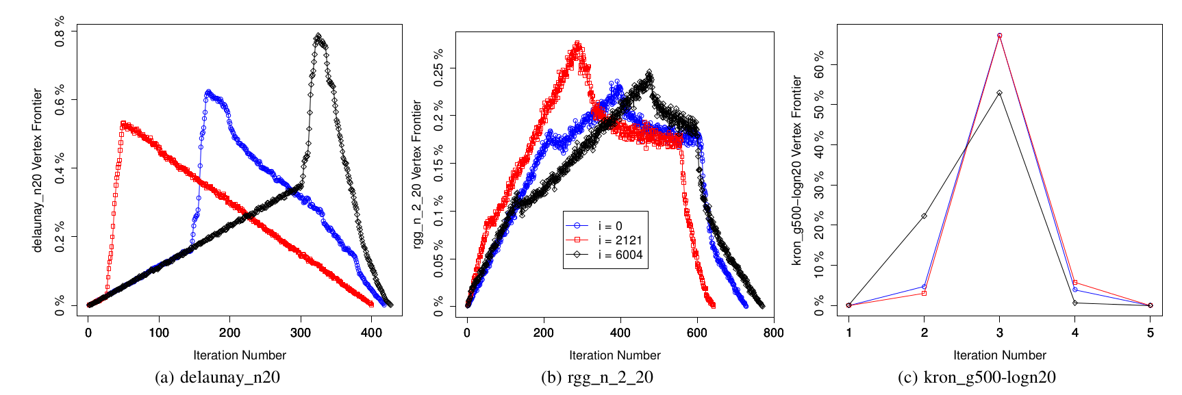
Figure 5 shows the evolution of vertex frontiers starting from three randomly chosen roots for three different types of graphs. We can see that traversals of high diameter graphs (such as road networks) tend to require a large number of iterations that each consist of a small amount of work. In contrast, for graphs with a small diameter (such as social networks) traversals require a small number of iterations consisting of a large amount of work.
It turns out that we can estimate the diameter of the graph by processing an initial batch of roots and storing the largest BFS distance seen from each of these roots. Since each root has a (roughly) equivalent amount of work, processing the first few hundred out of millions of total roots takes a trivial amount of the total execution time. We estimate the diameter to be the median of the stored distances and compare this value to a threshold. If the value exceeds the threshold, we continue to use the work-efficient approach because the graph is likely to have a large diameter. Otherwise, we switch to using the edge-parallel approach because the graph is likely to have a small diameter. More details on this sampling method can be found in our paper that is to be published at this year’s Supercomputing Conference in New Orleans.
Results
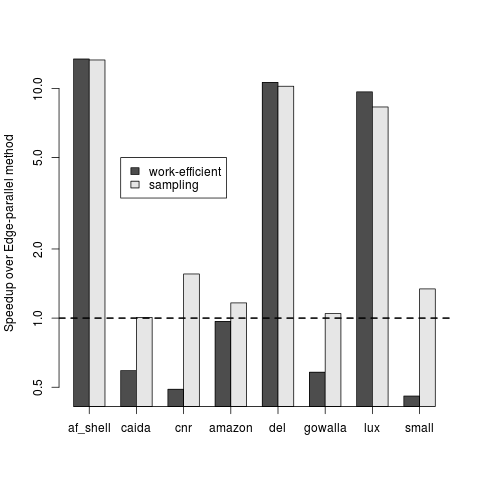
Figure 6 shows a comparison of the work-efficient and sampling methods to the edge-parallel method. For road networks and meshes (af_shell, del, and lux), these methods outperform the edge-parallel method by about 10x. For the remaining graphs our implementation improves upon previous work but sees more moderate speedups. Overall, the sampling approach performs 2.71x faster on average than the edge-parallel method.
Conclusion
In this post we discussed various ways to parallelize betweenness centrality calculations on the GPU. Since the structure of real-world graphs can vary tremendously, no single decomposition of threads to tasks provides peak performance for all input. For high-diameter graphs, using asymptotically efficient algorithms is paramount to obtaining high performance, whereas for low-diameter graphs it is preferable to maximize memory throughput, even at the cost of unnecessary memory accesses.
The importance of robust, high-performance primitives cannot be overstated for the implementation of more complicated parallel algorithms. Fortunately, libraries such as Thrust and CUB provide fast and performance portable building blocks to allow CUDA developers to tackle more challenging tasks.