[Note: Thejaswi Rao also contributed to the code optimizations shown in this post.]
Today NVIDIA released CUDA 7.5, the latest release of the powerful CUDA Toolkit. One of the most exciting new features in CUDA 7.5 is new Instruction-Level Profiling support in the NVIDIA Visual Profiler. This powerful new feature, available on Maxwell (GM200) and later GPUs, helps pinpoint performance bottlenecks, letting you quickly identify the specific lines of source code (and assembly instructions) limiting the performance of GPU code, along with the underlying reason for execution stalls.
In this post, I demonstrate Instruction-Level Profiling by showing how it helped understand and improve the performance limitations of a CUDA kernel that implements the Iterative Closest Point algorithm (the original source code, by Thomas Whelan, is available on Github). I’ll show how instruction-level profiling makes it easier to apply advanced optimizations, helping speed up the example kernel by 2.7X on an NVIDIA Quadro M6000 GPU.
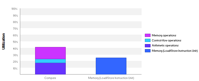
Profiling the kernel using the Guided Analysis feature of the Visual Profiler showed that the kernel performance was bound by instruction and memory latency. Latency issues indicate that the hardware resources are not used efficiently since most warps are stalled by a dependency on a data value from a previous math or memory instruction. Figure 1 shows that the compute units are only 40% utilized and memory units are around 25% utilized, so there is definitely room for improvement.
Stall Analysis in Previous Profiler Versions
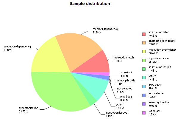
Before CUDA 7.5, the Visual Profiler was only capable of pointing out performance issues at the application or CUDA kernel level. For stall latency analysis, the CUDA 7.0 Visual Profiler produces the pie chart in Figure 2 by collecting various stall reason events for the entire kernel.
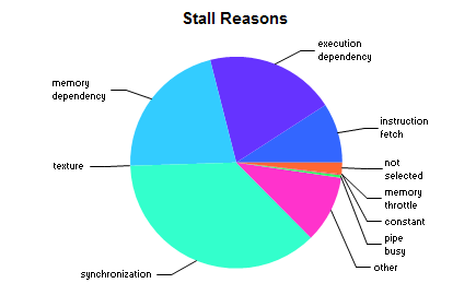
This pie chart shows that the two primary stall reasons in this kernel are synchronization and memory dependencies. But if I look into the kernel code, there are lots of memory accesses and __syncthreads() calls, so this high-level analysis doesn’t provide any specific insight into which instructions are potential bottlenecks. In general it can be very difficult to find exact bottleneck causes in complex kernels using kernel-level profiling analysis. This is where CUDA 7.5 can help, as you’ll see.
Instruction-Level Profiling
Instruction-level profiling in CUDA 7.5 uses program counter (PC) sampling with a per-streaming-multiprocessor (SM) fixed-frequency sampler. At each sample period, the collector picks an active warp from the SM and captures the warp’s PC and warp state. Warp selection is performed round-robin across all active warps on the SM.
Assuming there are 8 active warps on each SM warp scheduler and the sampling period is 256 cycles, the profiler collects samples as Figure 3 shows.
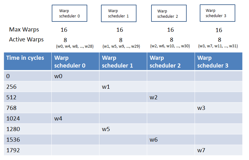
In the Visual Profiler, the sampling period is fixed from run to run on a given GPU, but it can vary across different GPUs.
Visual Profiler PC Sampling Results View
The Visual Profiler shows the Instruction-level profiling view when you select “Kernel Profile – PC sampling”. This view shows the distribution of samples across CUDA functions including kernels, non-inlined device functions and child kernels (launched via Dynamic Parallelism). It also lists the files containing the sampled GPU code. Figure 4 shows the output for the Iterative Closest Point example, where a single kernel is profiled (the kernel calls only inlined functions).

The view also contains a pie chart of warp state distribution as Figure 5 shows. The pie chart in this view statistically matches the stall reasons pie chart in Figure 2 that was produced using event collection.
Clicking on a function or file in the results opens the source-assembly view, as Figure 6 shows. The source-assembly view presents the warp state samples as a stacked bar graph next to the source line and instruction associated with the Program Counter in the sample. Hovering the mouse pointer over the stacked bar shows a tooltip containing the sample count and stall reason count for the source line or instruction. The stall reasons are sorted in decreasing order.

Analyzing the PC Sampling Output
Clicking on “CombinedKernel…” in the “Cuda Functions” table under “Analysis Results” opens the source assembly view and jumps to the first hotspot in the kernel at source line 197. The two primary stall reasons are synchronization (51.1%) and memory dependency (34.1%), as Figure 7 highlights.

Reducing Memory Dependency Stalls
Examining the assembly instructions corresponding to the hot spot source line shows that memory stalls occur at instructions that use the result of earlier LDL (“load local”) instructions, and synchronization stalls occur at the instruction after a BAR.SYNC barrier instruction (__syncthreads()).
Source line 197 indexes the local (stack-allocated) array row, and the profiler shows that this line correlates to an LDL instruction. NVIDIA GPUs do not have indexed register files, so if a stack array is accessed with dynamic indices, the compiler must allocate the array in local memory. In the Maxwell architecture, local memory stores are not cached in L1 and hence the latency of local memory loads after stores is significant. To work around this, I decided to use individual local variables instead of indexed variables.
I replaced the local array with individual local variables and unrolled the ‘for’ loops to use the new local variables.
Original code:
float row[7]
//Initialize array row
int shift = 0;
__shared__ float smem[CTA_SIZE];
for (int i = 0; i < 6; ++i)        // rows
{
    #pragma unroll
    for (int j = i; j < 7; ++j)    // cols + b
    {
        __syncthreads ();
        smem[tid] = row[i] * row[j];
        __syncthreads ();

        reduce(smem);

        if (tid == 0)
            gbuf.ptr (shift++)[blockIdx.x + gridDim.x * blockIdx.y]
                = smem[0];
    }
}
New code:
float row0, row1, row2, row3, row4, row5, row6;
//Initialize all elements
#define UNROLL_REDUCE(val, buf)                                     \
    do {                                                            \
        smem[tid] = val;                                            \
            __syncthreads();                                        \
            reduce(smem);                                           \
            if (tid == 0)                                           \
                buf.ptr (shift++)[blockIdx.x + gridDim.x * blockIdx.y] \
                    = smem[0]; \
    } while(0)

UNROLL_REDUCE(row0*row0, gbuf);
UNROLL_REDUCE(row0*row1, gbuf);
UNROLL_REDUCE(row0*row2, gbuf);
UNROLL_REDUCE(row0*row3, gbuf);
UNROLL_REDUCE(row0*row4, gbuf);
This change removed all the memory dependency stalls due to local memory accesses, which reduced the kernel run time from 3.9ms to 2.3ms, giving a 1.6X improvement in performance.
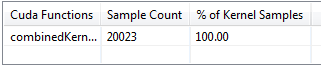
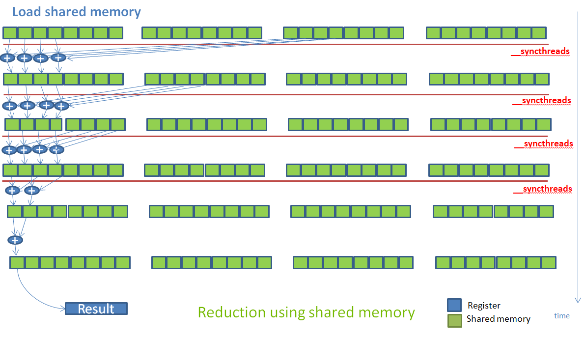
Figure 9 shows that memory dependency stalls reduced from 21.68% (Figure 5) to 8.21% (Figure 9) along with an overall sample count reduction from 30908 (Figure 4) to 20023 (Figure 8).
Reducing Synchronization Stalls
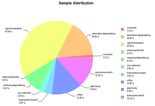
After the first optimization, Figure 9 shows that the kernel is bottlenecked by synchronization stalls, so I investigated how to reduce these next. Synchronization stalls occur when warps arrive at a barrier instruction and then wait for all other warps in the thread block to arrive. This kernel uses shared memory reductions, which introduce many barrier instructions, as Figure 10 illustrates.
The Parallel Forall post “Faster Parallel Reductions with Kepler” shows how reduction operations can be optimized using the shuffle instruction (available on the Kepler GPU architecture and later). I decided to use the same strategy on this kernel.
I modified the kernel to use shuffle instructions to implement intra-warp reductions first as Figure 11 shows. This reduced inter-warp synchronization and removed the need for many shared memory accesses, and therefore also eliminated multiple calls to __syncthreads().

Figure 12 shows the PC sampling distribution for the modified code, with a decrease in synchronization stalls, but an increase in execution dependency stalls.

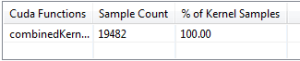
This optimization didn’t result in a significant performance increase; as you can see the total samples only went down from 20023 (Figure 8) to 19842 (Figure 13). Clicking on the kernel function again showed that line 93 has the maximum synchronization stalls as Figure 14 shows.
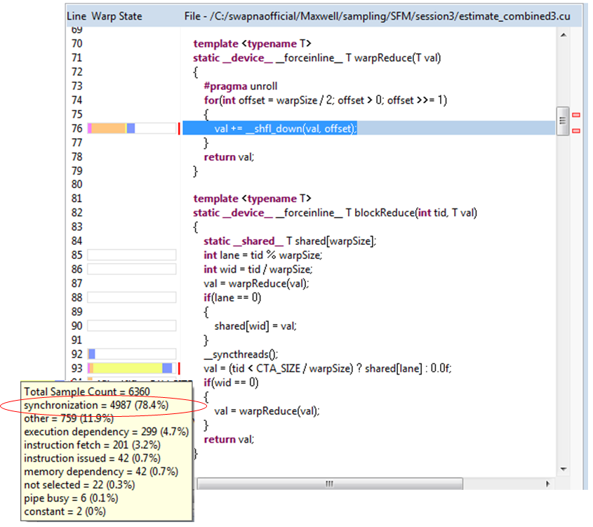
There is a shared store before the __syncthreads(), so it is evident that the stalls are due to shared memory store latency: all warps in the block wait for the shared store to complete. This wait happens for all 27 elements processed by each thread. Software pipelining is a common technique used to hide this sort of latency. The compiler cannot automatically perform software pipelining because it can’t reorder the code across __syncthreads(). Also, there is a global store after each reduction and the compiler can’t reorder the code across global loads/stores due to pointer aliasing issues. However, I know at the algorithm level that the elements each thread reduces do not depend on each other, so I modified the code to operate on multiple elements before syncing (manual software pipelining). Figure 15 shows the resulting code and sampling.

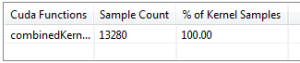
This indeed hides significant shared store latency, reducing synchronization samples from 4987 (Figure 14) to 2548 (Figure 15). It also results in a reduction of execution dependency stalls seen at line 76 as the second highest hotspot in figure 14. This is because the compiler now interleaves __shfl_down instructions for different elements while performing the intra-warp reduction. Checking the PC sampling output of this final code, now I see a significant reduction in the total number of samples from 19482 (Figure 13) to 13280 (Figure 16). The kernel time decreased from 2.33ms to 1.41ms.
Summary
The following table summarizes the samples collected, the stall reasons and the performance improvement achieved.
| Code version | Total Samples | Memory Dependency samples | Synchronization samples | Overallkernel time | Improvement |
| Original code | 30908 | 6490 (21.68%) | 10431 (33.75%) | 3.932ms | 1.0X |
| Reduced memory dependencies | 20039 | 1651 (8.24%) | 8213 (40.99%) | 2.333ms | 1.7X |
| Reduced synchronization stalls | 13230 | 1670 (12.63%) | 3991 (30.17%) | 1.418ms | 2.77X |
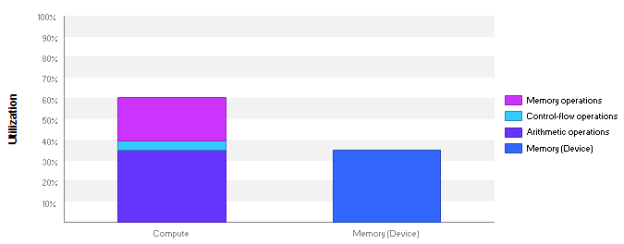
Thanks to the deep insight provided by Instruction-level profiling, I was able to decrease the kernel run time by 2.7X. Note that the Visual Profiler still shows latency as the limiter in the new code, but the compute and memory utilization have increased from 40% and 25% to 60% and 35%, respectively, as Figure 17 shows.
The NVIDIA Visual Profiler Instruction-level analysis features in CUDA 7.5 are very helpful for locating and fixing performance issues in CUDA code. You can read more about these features in the Profiler Users Guide.
Download CUDA 7.5 Today
CUDA Toolkit 7.5 is available now, so download it today! CUDA 7.5 is chock full of new features, including instruction-level profiling, mixed-precision (FP16) data storage, new cuSPARSE routines for accelerating natural language processing, and experimental support for GPU lambdas in C++. You can read all about it in the Parallel Forall post “New Features in CUDA 7.5“.
To learn more about the features in CUDA 7.5, register for the webinar “CUDA Toolkit 7.5 Features Overview” and put it on your calendar for September 22.