Speech recognition is an established technology, but it tends to fail when we need it the most, such as in noisy or crowded environments, or when the speaker is far away from the microphone. At Baidu we are working to enable truly ubiquitous, natural speech interfaces. In order to achieve this, we must improve the accuracy of speech recognition, especially in these challenging environments. We set out to make progress towards this goal by applying Deep Learning in a new way to speech recognition.
Deep Learning has transformed many important tasks; it has been successful because it scales well: it can absorb large amounts of data to create highly accurate models. Indeed, most industrial speech recognition systems rely on Deep Neural Networks as a component, usually combined with other algorithms. Many researchers have long believed that Deep Neural Networks (DNNs) could provide even better accuracy for speech recognition if they were used for the entire system, rather than just as the acoustic modeling component. However, it has proven difficult to find an end-to-end speech recognition system based on Deep Learning that improves on the state of the art.
Model and Data Co-design
One of the reasons this has been difficult is that training these networks on large datasets is computationally very intensive. The process of training DNNs is iterative: we instantiate ideas about models in computer code that trains a model, then we train the model on a training set and test it, which gives us new ideas about how to improve the model or training set. The latency of this loop is the rate limiting step that gates progress. Our models are relatively large, containing billions of connections, and we train them on thousands of hours of data, which means that training our models takes a lot of computation.
We choose our model sizes so that our models have the right amount of capacity to match our training dataset. If our model has too many parameters for our dataset, it will overfit the data: essentially using the excess capacity of the network to memorize training examples, which leads to a brittle model that performs well on the training set, but poorly on real-world data. Conversely, if our model has too few parameters for the dataset, it will underfit the data, which means the model fails to learn enough from the dataset. Therefore, choosing model size and dataset is a co-design process, where we incrementally increase the model size and obtain more training data. Arbitrarily increasing either generally leads to poor results.
Maximizing Strong Scaling
This observation determines how we use parallelism. Although our models are large, we can’t just weakly scale them to larger numbers of GPUs. We care primarily about strong scalability, because if we can get training to scale strongly with more GPUs, we can reduce the latency of our training process on model sizes that are relevant to our datasets. This allows us to come up with new ideas more quickly, driving progress.
Accordingly, we use multiple GPUs, working together, to train our models. GPUs are especially well suited for training these networks for a couple of reasons. Of course, we rely on the high arithmetic throughput and memory bandwidth that GPUs provide. But there are some other important factors: firstly, the CUDA programming environment is quite mature, and well-integrated into other HPC infrastructure, such as MPI and Infiniband, which makes us much more productive as we code our ideas into a system to train and test our models. CUDA libraries are also essential to this project: our system relies on both NVIDIA cuBLAS and cuDNN.
Secondly, because each GPU is quite powerful, we don’t have to over-partition our models to gain compute power. Finely partitioning our models across multiple processors is challenging, due to inefficiencies induced by communication latency as well as algorithmic challenges, which scale unfavorably with increased partitioning. Let me explain why this is the case.
When training models, we rely on two different types of parallelism, which are often called “model parallelism” and “data parallelism”. Model parallelism refers to parallelizing the model itself, distributing the neurons across different processors. Some models are easier to partition than others. As we employ model parallelism, the amount of work assigned to each processor decreases, which limits scalability because at some point, the processors are under-occupied.
We also use “data parallelism”, which in this context refers to parallelizing the training process by partitioning the dataset across processors. Although we have large numbers of training examples, scalability when using data parallelism is limited due to the need to replicate the model for each partition of the dataset, and consequently to combine information learned from each partition of the dataset to produce a single model.
How We Parallelize Our Model
Training neural networks involves solving a highly non-convex numerical optimization. Much research has been conducted to find the best algorithm for solving this optimization problem, and the current state of the art is to use stochastic gradient descent (SGD) with momentum. Although effective, this algorithm is particularly difficult to scale, because it favors taking many small optimization steps in sequence, rather than taking a few large steps. This implies examining a relatively small group of training examples at a time. We trained our speech recognition system on minibatches of 512 examples, each subdivided into microbatches of 128 examples. We processed on 8 Tesla K40s for each training instance in 4 separate pairs, using 4-way data parallelism and two-way model parallelism.
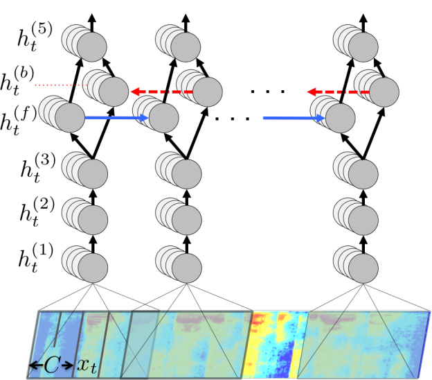
As shown in Figure 1, our model has 5 layers. The first layer is a convolutional layer that operates on an input spectrogram (a 2-D signal where one dimension represents frequency and the other time) and produces many 1-D responses, for each time sample. cuDNN’s ability to operate on non-square images with asymmetric padding made implementation of this layer simple and efficient. The next two layers and the final layer are fully connected, implemented using cuBLAS.
If our model were made with only these 4 layers, model parallelism would be fairly straightforward, since these layers are independent in the time dimension. However, the 4^th^ layer is responsible for propagating information along the time dimension. We use a bidirectional recurrent layer, where the forward and backward directions are independent. Because the recurrent layers require a sequential implementation of activations followed by non-linearity, they are difficult to parallelize. Traditional approaches like prefix-sum do not work, because the implied operator (matrix multiply followed by non-linearity) is extremely non-associative.
The bidirectional layer accounts for about 40% of the total training time, so parallelizing it is essential. We gain two-way model parallelism despite the sequential nature of recurrent neural networks by exploiting the independence of the forward and backward direction in the bidirectional recurrent layer. We divide the neuron responses in half along the time dimension, assigning each half to a GPU. For the recurrent layer, we have the first GPU process the forward direction, while the second processes the backward direction, until they both reach the partition at the center of the time dimension. They then exchange activations and switch roles: the first GPU processes the backward direction, while the second processes the forward direction.
Results: Advancing the State of the Art in Speech Recognition
Combining these techniques, we built a system that allows us to train our model on thousands of hours of speech data. Because we have been able to iterate quickly on our models, we were able to create a speech recognition system based on an end-to-end deep neural network that significantly improves on the state of the art, especially for noisy environments.
We attained a 16% word error rate on the full switchboard dataset, a widely used standard dataset where the prior best result was 18.4%. On a noisy test set we developed, we achieved a 19.1% word error rate, which compares favorably to the Google API, which achieved 30.5% error rate, Microsoft Bing, which achieved 36.1%, and Apple Dictation, which achieved a 43.8% error rate. Often, when commercial speech systems have low confidence in their transcription due to excessive noise, they refuse to provide any transcription at all. The above error rates were computed only for utterances on which all compared systems produced transcriptions, to give them the benefit of the doubt on more difficult utterances.
In summary, the computational resources afforded by GPUs, coupled with simple, scalable models, allowed us to iterate more quickly on our large datasets, leading to a significant improvement in speech recognition accuracy. We were able to show that speech recognition systems built on deep learning from input to output can outperform traditional systems built with more complicated algorithms. We believe that with more data and compute resources we will be able to improve speech recognition even further, working towards the goal of enabling ubiquitous, natural speech interfaces.
Learn more at GTC 2015
If you’re interested in learning more about this work, come see our GTC 2015 talk “Speech: The Next Generation” at 3PM Tuesday, March 17 in room 210A of the San Jose Convention Center (session S5631), or read our paper.
With dozens of sessions on Machine Learning and Deep Learning, you’ll find that GTC is the place to learn about machine learning in 2015! Readers of Parallel Forall can use the discount code GM15PFAB to get 20% off any conference pass!