Histograms are an important data representation with many applications in computer vision, data analytics and medical imaging. A histogram is a graphical representation of the data distribution across predefined bins. The input data set and the number of bins can vary greatly depending on the domain, so let’s focus on one of the most common use cases: an image histogram using 256 bins for each color channel. Even though we’ll use a specific problem setup the same algorithms can benefit other computational domains as well.
A basic serial image histogram computation is relatively simple. For each pixel of the image and for each RGB color channel we find a corresponding integer bin from 0 to 255 and increment its value. Atomic operations are a natural way of implementing histograms on parallel architectures. Depending on the input distribution, some bins will be used much more than others, so it is necessary to support efficient accumulation of the values across the full memory hierarchy. This is similar to reduction and scan operations, but the main challenge with histograms is that the output location for each element is not known prior to reading its value. Therefore, it is impossible to create a generic parallel accumulation scheme that completely avoids collisions. Histograms are now much easier to handle on GPU architectures thanks to the improved atomics performance in Kepler and native support of shared memory atomics in Maxwell.
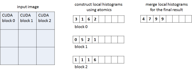
Our histogram implementation has two phases and two corresponding CUDA C++ kernels, as Figure 1 shows. In the first phase each CUDA thread block processes a region of the image and accumulates a corresponding local histogram, storing the local histogram in global memory at the end of the phase. The second kernel accumulates all per-block histograms into the final histogram stored in global memory. The work separation between blocks in the first phase reduces contention when accumulating values into the same bin.
For the first kernel we explored two implementations: one that stores per-block local histograms in global memory, and one that stores them in shared memory. Using the shared memory significantly reduces the expensive global memory traffic but requires efficient hardware for shared memory atomics. We compare the two approaches to investigate performance differences on the Kepler and Maxwell architectures.
Here is a sample kernel code for per-block accumulation using global atomics.
__global__ void histogram_gmem_atomics(const IN_TYPE *in, int width, int height, unsigned int *out)
{
  // pixel coordinates
  int x = blockIdx.x * blockDim.x + threadIdx.x;
  int y = blockIdx.y * blockDim.y + threadIdx.y;

  // grid dimensions
  int nx = blockDim.x * gridDim.x;
  int ny = blockDim.y * gridDim.y;

  // linear thread index within 2D block
  int t = threadIdx.x + threadIdx.y * blockDim.x;

  // total threads in 2D block
  int nt = blockDim.x * blockDim.y;

  // linear block index within 2D grid
  int g = blockIdx.x + blockIdx.y * gridDim.x;

  // initialize temporary accumulation array in global memory
  unsigned int *gmem = out + g * NUM_PARTS;
  for (int i = t; i < 3 * NUM_BINS; i += nt) gmem[i] = 0;

  // process pixels
  // updates our block's partial histogram in global memory
  for (int col = x; col < width; col += nx)
    for (int row = y; row < height; row += ny) {
      unsigned int r = (unsigned int)(256 * in[row * width + col].x);
      unsigned int g = (unsigned int)(256 * in[row * width + col].y);
      unsigned int b = (unsigned int)(256 * in[row * width + col].z);
      atomicAdd(&gmem[NUM_BINS * 0 + r], 1);
      atomicAdd(&gmem[NUM_BINS * 1 + g], 1);
      atomicAdd(&gmem[NUM_BINS * 2 + b], 1);
    }
}
The shared atomics version is similar. The main difference is the temporary array storage and the copy of the local histogram into global memory.
__global__ void histogram_smem_atomics(const IN_TYPE *in, int width, int height, unsigned int *out)
{
  // pixel coordinates
  int x = blockIdx.x * blockDim.x + threadIdx.x;
  int y = blockIdx.y * blockDim.y + threadIdx.y;

  // grid dimensions
  int nx = blockDim.x * gridDim.x;
  int ny = blockDim.y * gridDim.y;

  // linear thread index within 2D block
  int t = threadIdx.x + threadIdx.y * blockDim.x;

  // total threads in 2D block
  int nt = blockDim.x * blockDim.y;

  // linear block index within 2D grid
  int g = blockIdx.x + blockIdx.y * gridDim.x;

  // initialize temporary accumulation array in shared memory
  __shared__ unsigned int smem[3 * NUM_BINS + 3];
  for (int i = t; i < 3 * NUM_BINS + 3; i += nt) smem[i] = 0;
  __syncthreads();

  // process pixels
  // updates our block's partial histogram in shared memory
  for (int col = x; col < width; col += nx)
    for (int row = y; row < height; row += ny) {
      unsigned int r = (unsigned int)(256 * in[row * width + col].x);
      unsigned int g = (unsigned int)(256 * in[row * width + col].y);
      unsigned int b = (unsigned int)(256 * in[row * width + col].z);
      atomicAdd(&smem[NUM_BINS * 0 + r + 0], 1);
      atomicAdd(&smem[NUM_BINS * 1 + g + 1], 1);
      atomicAdd(&smem[NUM_BINS * 2 + b + 2], 1);
    }
  __syncthreads();

  // write partial histogram into the global memory
  out += g * NUM_PARTS;
  for (int i = t; i < NUM_BINS; i += nt) {
    out[i + NUM_BINS * 0] = smem[i + NUM_BINS * 0];
    out[i + NUM_BINS * 1] = smem[i + NUM_BINS * 1 + 1];
    out[i + NUM_BINS * 2] = smem[i + NUM_BINS * 2 + 2];
  }
}
In the second kernel we accumulate all partial histograms into the global one. This kernel is the same for both global and shared atomics implementations.
__global__ void histogram_final_accum(const unsigned int *in, int n, unsigned int *out)
{
  int i = blockIdx.x * blockDim.x + threadIdx.x;
  if (i < 3 * NUM_BINS) {
    unsigned int total = 0;
    for (int j = 0; j < n; j++)
      total += in[i + NUM_PARTS * j];
    out[i] = total;
  }
}
Now let’s pick a few interesting test cases to harness our GPU implementation. To cover a spectrum of input data, we split our test images into two categories: synthetic and real-world images.
The first data set represents random color distributions with varying entropy. In these tests we generate random distributions with progressively more histogram bin collisions. For example, 100% entropy means all bins have equal probability and this is arguably the best scenario for the atomics implementation. 0% entropy represents all-to-one collision type with equal values for all pixels. This is the worst case scenario for atomics since all threads are trying to write to the same address.
Aside from synthetic tests, it makes sense to include real images in our benchmarks as well, because they are more likely to represent memory access patterns seen in real world histogram applications. As you can see in the photos below there are usually some regions with similar color patterns. These regions can generate many collisions for atomic operations to challenge our approach.


Figures 2 and 3 show the benchmarking results for two image sets on Kepler (GeForce GTX TITAN, GK100) and Maxwell (GeForce GTX TITAN X, GM200) architectures respectively. Each image has the same resolution of 1080p. The plots show timings for our two implementations compared across various input sets.
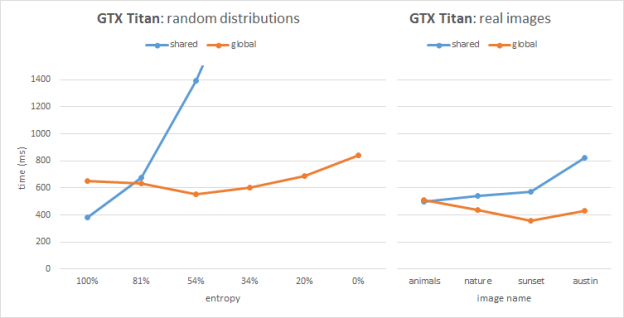
As we can see from the Kepler performance plots, the global atomics perform better than shared in most cases, except the images with high entropy. The Kepler architecture improved (vs. the previous Fermi architecture) global memory atomics performance by resolving conflicts in L2. On the other hand, Kepler emulates shared memory atomics in software, and high collision tests and real images suffer from serialization issues. In the 100% entropy case (white noise) we have perfect bin distribution and atomic conflicts do not play a significant role in performance; in this special case the shared memory version helps save bandwidth and outperforms the global atomics.
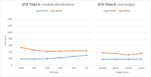
On Maxwell the global atomics implementation performs similarly compared to Kepler. However the Maxwell architecture features hardware support for shared memory atomics and we can clearly see that in all cases the shared atomics version performs best. The shared atomics histogram implementation is almost 2x faster than the global atomics version on Maxwell. Moreover, the performance is very stable across different workloads including both synthetic and real images. This stable performance is very important in real-time histogram applications in computer vision.
To summarize, histograms are easy to implement with shared memory atomics. This approach can attain high performance on Maxwell due to its native support for shared atomics. It is also possible to improve the histogram performance by additionally compressing the bin identifiers into {bin_id, count} pairs for each thread using RLE encoding. This technique reduces the size of the aggregation problem and provides a speed-up over the standard shared/global atomic implementations. All histogram experiments are available in the experimental master branch of the CUB library.