In this blog post I will briefly discuss the importance and simplicity of graph coloring and its application to one of the most common problems in sparse linear algebra – the incomplete-LU factorization. My goal is to convince you that graph coloring is a problem that is well-suited for GPUs and that it should be viewed as a tool that can be used to expose latent parallelism even in cases where it is not obvious. In fact, I will apply this tool to expose additional parallelism in one of the most popular black-box preconditioners/smoothers—the incomplete-LU factorization—which is used in many applications, including Computational Fluid Dynamics; Computer-Aided Design, Manufacturing, and Engineering (CAD/CAM/CAE); and Seismic Exploration (Figure 1).

What is Graph Coloring?
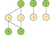
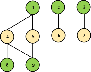
In general, graph coloring refers to the problem of finding the minimum number of colors that can be used to color the nodes of a graph, such that no two adjacent (connected) nodes have the same color. For example, the graph in Figure 2 can be colored with two colors (green and yellow).
Why is this mathematical problem of interest to us? Well, imagine that each node in the graph represents a task and each edge represents a dependency between two tasks. Then, graph coloring tells us which tasks are independent. Assuming that the edges have no particular direction assigned to them, we can process the tasks with the same color in parallel (they are independent by construction), perform a barrier, and proceed to the next set of tasks that are identified by a different color. Not all problems can be mapped to such a framework, but many are amenable to it.
The next question we should answer is how difficult is it to perform graph coloring? Now that the cuSPARSE routine provides a graph coloring implementation in the csrcolor() routine, for most users it is trivially easy. But in this post I want to talk about implementing the algorithm itself in a bit more detail.
It is well-known that finding the best solution to this problem is NP-complete. However, there are many parallel algorithms that can find an approximate solution very quickly. Indeed, the exact solution is often not even required, as long as we obtain enough parallelism to fully utilize our parallel computing platform.
A Parallel Algorithm for Graph Coloring
The typical parallel algorithm for finding the approximate graph coloring is based on Luby’s maximal independent set algorithm. In this algorithm we
- assign a random number to each node;
- find an independent set by selecting nodes that have the maximum value among neighbors;
- (potentially) iterate on the remaining nodes until no more can be added to the independent set.
The third step allows us to find the maximal independent set, but graph coloring works even if we only find an independent set, although it will require more colors. The nodes in the (maximal) independent set can be assigned the same color, and the algorithm proceeds in the same fashion to color the remaining nodes of the graph.
The following code sample shows a CUDA C++ kernel for finding an independent set from an adjacency matrix of a graph stored in compressed sparse row (CSR) format, where Ao contains the matrix row offsets, Ac contains the column indices and Av contains the non-zero values.
#include <thrust/count.h>

__global__ void color_jpl_kernel(int n, int c, const int *Ao,
                                 const int *Ac, const double *Av,
                                 const int *randoms, int *colors)
{
  for (int i = threadIdx.x+blockIdx.x*blockDim.x;
       i < n;
       i += blockDim.x*gridDim.x)
  {
    bool f=true; // true iff you have max random

    // ignore nodes colored earlier
    if ((colors[i] != -1)) continue;

    int ir = randoms[i];

    // look at neighbors to check their random number
    for (int k = Ao[i]; k < Ao[i+1]; k++) {
      // ignore nodes colored earlier (and yourself)
      int j = Ac[k];
      int jc = colors[j];
      if (((jc != -1) && (jc != c)) || (i == j)) continue;
      int jr = randoms[j];
      if (ir <= jr) f=false;
    }

    // assign color if you have the maximum random number
    if (f) colors[i] = c;
  }
}

#define CUDA_MAX_BLOCKS <Maximum blocks to launch, depends on GPU>

void color_jpl(int n,
               const int *Ao, const int *Ac, const double *Av,
               int *colors)
{
    int *randoms; // allocate and init random array
    thrust::fill(colors, colors+n, -1); // init colors to -1

    for(int c=0; c < n; c++) {
        int nt = 256;
        int nb = min((n + nt - 1)/nt,CUDA_MAX_BLOCKS);
        color_jpl_kernel<<<nb,nt>>>(n, c,
                                    Ao, Ac, Av,
                                    randoms,
                                    colors);
        int left = (int)thrust::count(colors,colors+n,-1);
        if (left == 0) break;
    }
}
Luby’s algorithm is very powerful because it provides an outline that can be adjusted for different purposes using different heuristics. For example, we can use multiple hash functions instead of random numbers to assign multiple colors at once in order to perform the graph coloring faster. We can also attempt to use the degree (number of in/out edges) of a node in combination with a random number to color nodes with larger/smaller degree first, which could potentially allow us to perform reordering that minimizes fill-in and exposes additional parallelism. Many such combinations are still open research problems.
Another interesting aspect of this parallel outline is that it is ideally suited for GPUs. It is very easy to map the available parallelism to the CUDA programming model. For example, each CUDA thread can look only at its local neighbors and essentially perform the color assignment independently of others.
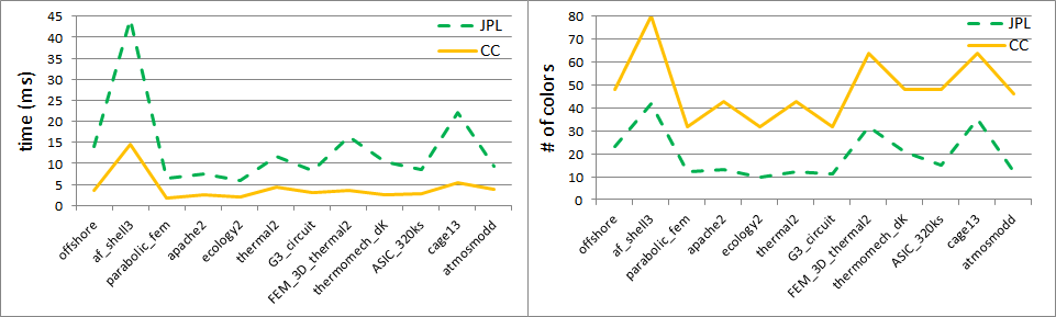
Figure 3 illustrates the performance of the above algorithm on several sample problems with two different heuristics based on the original idea about random numbers (Jones-Plassmann-Luby) and the novel idea about multiple hash functions (Cohen-Castonguay). The experiments were performed with CUDA Toolkit 7.0 on Ubuntu 14.04 LTS, on an NVIDIA Tesla K40c GPU Accelerator. For more details please refer to our technical report [1].
Applying Graph Coloring to Incomplete-LU factorization
The incomplete-LU factorization is an algorithm that approximately factors a large sparse matrix 


This approximation is later used as an iterative method preconditioner or an algebraic multigrid smoother, and is designed to speed up convergence to the solution of a given linear system.
In order to find the
If we performed the above algorithm in dense storage, we would simply compute the LU-factorization without pivoting (ignore the diagonal boosting for now). However, in sparse storage the algorithm is more complex. Notice that as we proceed with Gaussian elimination, the matrix 
The incomplete-LU factorization simply drops the extra elements created during the Gaussian elimination process. Different heuristics for dropping the elements result in different types of incomplete-LU, such as ILU0, ILUT and ILU(p). We focus on the incomplete-LU with 0 fill-in (ILU0), where all extra elements outside of the sparsity pattern of the original matrix
On one hand, in order to parallelize this algorithm, we can analyze the dependencies between rows, and find out which rows can be processed in parallel. For example, for a given coefficient matrix

the dependencies between rows are represented by the directed acyclic graph (DAG) in Figure 4.
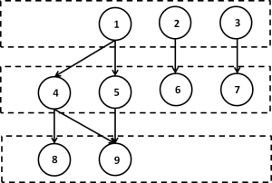
Notice that it is identical to the graph on which we performed graph coloring in Figure 2. Here the independent rows are organized into levels and this parallel approach is called level scheduling.
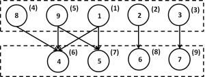
On the other hand, we can explicitly reorder the matrix a priori based on graph coloring (such that nodes with the same color are ordered next to each other) and only then analyze it for parallelism. The reordered matrix based on the coloring from the previous section is shown below.
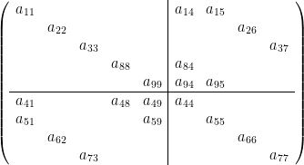
It turns out that reordering based on graph coloring exposes additional parallelism, making the dependency dag shorter and wider. This means fewer colors, which means fewer parallel stages with greater parallelism in each stage.
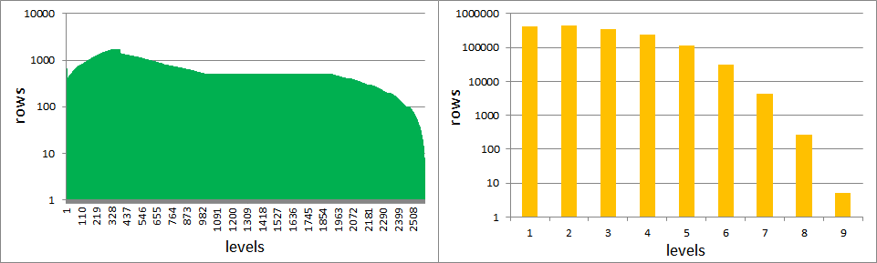
In fact, for realistic matrices we can have up to 100 times more rows per level after performing reordering based on graph coloring, as Figure 6 illustrates.
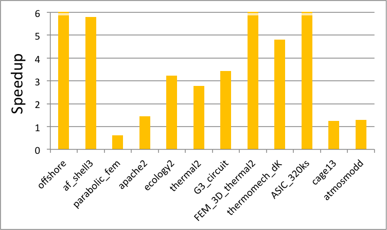
Ultimately, as a result of graph coloring we are able to better utilize the GPU. Indeed, we can now take full advantage of its memory bandwidth because we have exposed enough parallelism in our problem. We show the resulting improvement in performance on a sample set of matrices in Fig. 7, where we have used the coloring algorithm implemented in the cuSPARSE library csrcolor() routine. The experiments were performed with CUDA Toolkit 7.0 on Ubuntu 14.04 LTS, on an NVIDIA Tesla K40c GPU Accelerator. For more details please refer to the technical report [1].
Finally, note that we have used approximate graph coloring, and therefore could potentially further improve the performance of ILU0 with better heuristics or re-coloring techniques.
Conclusion
Graph coloring is a general technique that can enable greater parallelism to be extracted from a problem. As an example, I have shown that reordering matrix rows based on graph coloring can provide a significant speedup of the to the incomplete-LU factorization algorithm on the GPU. Also, I have shown that parallel approximate graph coloring itself is well suited for the GPU. In fact, the algorithm parallelizes extremely well and can be adapted to a variety of problems by using different heuristics.
References
[1] M.Naumov, P.Castonguay, J. Cohen, “Parallel Graph Coloring with Applications to the incomplete-LU factorization on the GPU”, NVIDIA Research Technical Report, May, 2015.