In this post, I will discuss techniques you can use to maximize the performance of your GPU-accelerated MATLAB® code. First I explain how to write MATLAB code which is inherently parallelizable. This technique, known as vectorization, benefits all your code whether or not it uses the GPU. Then I present a family of function wrappers—bsxfun, pagefun, and arrayfun—that take advantage of GPU hardware, yet require no specialist parallel programming skills. The most advanced function, arrayfun, allows you to write your own custom kernels in the MATLAB language.
If these techniques do not provide the performance or flexibility you were after, you can still write custom CUDA code in C or C++ that you can run from MATLAB, as discussed in our earlier Parallel Forall posts on MATLAB CUDA Kernels and MEX functions.
All of the features described here are available out of the box with MATLAB and Parallel Computing Toolbox™.
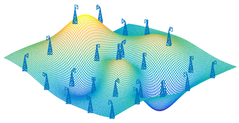
Mobile phone signal strength example
Throughout this post, I will use an example to help illustrate the techniques. A cellular phone network wants to map its coverage to help plan for new antenna installations. We imagine an idealized scenario with M = 25 cellphone masts, each H = 20 meters in height, evenly spaced on an undulating 10km x 10km terrain. Figure 1 shows what the map looks like.
On the GPU, in the following listing we define a number of variables including:
- map: An N x 3 height field in a 10km x 10km grid (N = 10,000);
- masts: An M x 3 array of antenna positions, at height H;
- AntennaDirection: A 3 x M array of vectors representing the orientation of each antenna.
% Map definition
gridpts = linspace(-5, 5, 100);
[mapX, mapY] = meshgrid(gridpts*1000);
N = numel(mapX);
% Procedurally generated terrain
mapZ = 100 * (peaks(gridpts/2) + 0.3*peaks(gridpts/2)' + flipud(peaks(gridpts/6)));

% Antenna masts - index into map spacing every 20 gridpoints
index = 1:20:100;
mastX = mapX(index, index);
mastY = mapY(index, index);
H = 20; % All masts are 20 meters in height
mastZ = mapZ(index, index) + H;
% Antenna properties
M = numel(mastX);
Frequency = 800e6;         % 800 MHz transmitters
Power = 100 * ones(1, M);  % Most transmitters use 100 W of power
Power(1:4:M) = 400;        % A few transmitters are more powerful
Power([3 14 22]) = 0;      % A small number are out of order
% Finally, give each antenna a random orientation. This is represented by
% horizontal vectors representing the direction the antennae are facing.
AntennaAngle = rand(1, M) * 2*pi;
AntennaDirection = [cos(AntennaAngle); sin(AntennaAngle); zeros(1, M)];

% Set up some random rotation matrices, stacked along the 3rd
% dimension as 3 x 3 x M arrays
tiltAngle = gpuArray.rand([1 1 M])*360;
Zero = gpuArray.zeros([1 1 M]);
One  = gpuArray.ones([1 1 M]);
Tilt = [One  Zero             Zero;
        Zero cosd(tiltAngle) -sind(tiltAngle);
        Zero sind(tiltAngle)  cosd(tiltAngle)];
turnAngle = gpuArray.rand([1 1 M])*360;
Pan = [cosd(turnAngle)  -sind(turnAngle) Zero;
       sind(turnAngle)   cosd(turnAngle) Zero;
       Zero              Zero            One];

% Set up indices into the data
mapIndex = gpuArray.colon(1,N)'; % N x 1 array of map indices
mastIndex = gpuArray.colon(1,M); % 1 x M array of mast indices
[RowIndex, ColIndex] = ndgrid(mapIndex, mastIndex);

% Put the map data on the GPU and concatenate the map
% positions into a single 3-column matrix containing all
% the coordinates [X, Y, Z].
map = gpuArray([mapX(:) mapY(:) mapZ(:)]);
masts = gpuArray([mastX(:) mastY(:) mastZ(:)]);
AntennaDirection = gpuArray(AntennaDirection);
Vectorization basics
Computational hot spots in code generally appear as loops or repeated segments of code, where the repeated operations are naturally parallel; in other words, they don’t depend on each other. The simplest approach to vectorization in MATLAB is to take advantage of matrix algebra in your mathematical operations. Let’s say I need to rotate all the antennae downwards by 10 degrees, as the following code shows.
% 3D rotation around the X axis
Elevation = [1        0         0;
             0 cosd(10) -sind(10);
             0 sind(10)  cosd(10)];
% Allocate a new array of directions and loop through to compute them
NewAntennaDirection = gpuArray.zeros(size(AntennaDirection));
for ii = 1:M
    NewAntennaDirection(:,ii) = Elevation * AntennaDirection(:,ii);
end
Note, however, that there’s no dependency between one rotation and the next. The rules of matrix multiplication let me do this without a loop.
AntennaDirection = Elevation * AntennaDirection;
This code runs a lot faster, especially on the GPU which was crippled by very low utilization in the serial code (we were asking it to do too little work at a time).
Calculating Signal Strength
The following code calculates the peak signal strength at each grid point on the map by measuring the losses between the grid point and the transmitters. It loops over every grid point and every antenna, computing one value per grid point. Since modern cell phones are in communication with multiple transmitters at once, the code averages the three strongest signals. To add some additional real-world complexity to the calculation, antennae that are pointing away from the location cannot be included (the signal strength is effectively zero).
% Allocate GPU memory for results
signalMap = gpuArray.zeros(size(mapX));
signalPowerDecibels = gpuArray.zeros(M, 1);

% Outer loop over the grid points
NN = 10; % This version is too slow to process more than a few points
for ii = 1:NN

    % Get the power received from every mast at this grid point
    for jj = 1:M

        % Calculate the distance from map position ii to antenna jj
        pathToAntenna = masts(jj,:) - map(ii,:);
        distance = sqrt(sum(pathToAntenna).^2);

        % Apply the free space path loss formula to the antenna power
        pathLoss = (4 .* pi .* distance * Frequency ./ 3e8).^2;
        signalPowerWatts = Power(jj) ./ pathLoss;

        % Convert to decibels (dBm)
        signalPowerDecibels(jj) = 30 + 10 * log10(signalPowerWatts);

        % Reset the power to zero if the antenna is not facing this way.
        % We can tell this from the dot product.
        directionDotProduct = dot(pathToAntenna, AntennaDirection(:,jj));
        if directionDotProduct < 0
            signalPowerDecibels(jj) = -inf; % 0 Watts = -inf decibels
        end

    end

    % Sort the power from each mast
    signalPowerSorted = sort(signalPowerDecibels, 'descend');
    % Strength is the average of the three strongest signals
    signalMap(ii) = mean(signalPowerSorted(1:3));
end
If we time this code, we get the following.
Signal strength compute time per gridpoint using loops = 37.4768ms
First I’ll focus on pulling the basic algebra out of the loop. Scalar operators like .* and sqrt work on larger arrays in an element-by-element manner. Reductions, like sum and mean, can work along a chosen dimension of an N-dimensional input. Using these features and reshaping the data allows us to remove the loops.
First I’ll reshape the data. At the moment, there are two lists of points, with each row representing one point, and the first column representing the 


X = reshape(map, [], 1, 3);
A = reshape(masts, 1, [], 3);
Let ![X_i = [X^x_i, X^y_i, X^z_i]](https://s0.wp.com/latex.php?latex=X_i+%3D+%5BX%5Ex_i%2C+X%5Ey_i%2C+X%5Ez_i%5D&bg=transparent&fg=000&s=0&c=20201002)

![A_j = [A^x_j, A^y_j, A^z_j]](https://s0.wp.com/latex.php?latex=A_j+%3D+%5BA%5Ex_j%2C+A%5Ey_j%2C+A%5Ez_j%5D&bg=transparent&fg=000&s=0&c=20201002)

![X = \left[ \begin{array}{c} X_1 \\ X_2 \\ \vdots \\ X_N \end{array} \right], ~~ A = \left[ \begin{array}{cccc} A_1 & A_2 & \cdots & A_M \end{array} \right].](https://s0.wp.com/latex.php?latex=X+%3D+%5Cleft%5B+%5Cbegin%7Barray%7D%7Bc%7D+X_1+%5C%5C+X_2+%5C%5C+%5Cvdots+%5C%5C+X_N+%5Cend%7Barray%7D+%5Cright%5D%2C+%7E%7E+A+%3D+%5Cleft%5B+%5Cbegin%7Barray%7D%7Bcccc%7D+A_1+%26+A_2+%26+%5Ccdots+%26+A_M+%5Cend%7Barray%7D+%5Cright%5D.&bg=transparent&fg=000&s=0&c=20201002)
I want to create a matrix of size N x M which contains the distance of every grid point to every antenna. Conceptually, I want to replicate the map data along the columns, and the antenna data along the rows, and subtract the two arrays to get the path vectors from grid points to antennae:
![\left[ \begin{array}{llll}A_1 & A_2 & \cdots & A_M \\[0.7em] \vdots & \vdots & \vdots & \vdots \\[0.7em] A_1 & A_2 & \cdots & A_M \end{array} \right] - \left[ \begin{array}{lll} X_1 & \cdots & X_1 \\ X_2 & \cdots & X_2 \\ \vdots & \cdots & \vdots \\ X_N & \cdots & X_N \end{array} \right].](https://s0.wp.com/latex.php?latex=%5Cleft%5B+%5Cbegin%7Barray%7D%7Bllll%7DA_1+%26+A_2+%26+%5Ccdots+%26+A_M+%5C%5C%5B0.7em%5D+%5Cvdots+%26+%5Cvdots+%26+%5Cvdots+%26+%5Cvdots+%5C%5C%5B0.7em%5D+A_1+%26+A_2+%26+%5Ccdots+%26+A_M+%5Cend%7Barray%7D+%5Cright%5D+-+%5Cleft%5B+%5Cbegin%7Barray%7D%7Blll%7D+X_1+%26+%5Ccdots+%26+X_1+%5C%5C+X_2+%26+%5Ccdots+%26+X_2+%5C%5C+%5Cvdots+%26+%5Ccdots+%26+%5Cvdots+%5C%5C+X_N+%26+%5Ccdots+%26+X_N+%5Cend%7Barray%7D+%5Cright%5D.&bg=transparent&fg=000&s=0&c=20201002)
I could do this using repmat:
pathToAntenna = repmat(A, [N, 1, 1]) - repmat(X, [1, M, 1]);
However, this is actually doing unnecessary work and taking up extra memory. I’ll introduce the function bsxfun, the first in a family of essential function wrappers useful for high-performance coding. bsxfun applies a binary (two-input) operation (such as minus in this case), expanding along any dimensions that don’t match between the two arguments as it goes, extending the normal rules for scalars.
pathToAntenna = bsxfun(@minus, A, X);
Computing the path loss involves scalar operations that work independently on each element of an array (known as element-wise), plus sum to add the x, y and z values along the 3rd dimension.
distanceSquared = sum(pathToAntenna.^2, 3); % Syntax to sum along dim 3
distance = sqrt(distanceSquared);
pathLoss = (4 .* pi .* distance .* Frequency ./ 3e8).^2;
The power and dot product calculations can also be done using combinations of bsxfun, sum, and element-wise arithmetic.
% Power calculation
signalPowerWatts = bsxfun(@rdivide, Power, pathLoss);
signalPowerDecibels = 30 + 10 * log10(signalPowerWatts);

% Dot product is just the sum along X,Y,Z of two arrays multiplied
dirn = permute(AntennaDirection, [3 2 1]); % Permute to 1 x M x 3
directionDotProduct = sum(bsxfun(@times, pathToAntenna, dirn), 3);
The original looping code included a conditional statement to set the power to zero (or 
isFacing = directionDotProduct >= 0;
This is a mask identifying every entry in the data to be included in the calculation. What’s more, it can be used to index all the invalid entries and set them to
signalPowerDecibels(~isFacing) = -inf;
Finally, to compute the signal strength I tell sort and mean to operate along rows.
signalPowerSorted = sort(signalPowerDecibels, 2, 'descend');
signalMap = mean(signalPowerSorted(:,1:3), 2);
Even for this relatively small amount of data (for a GPU application) there is a significant speed-up. This is partly because the GPU was being used so inefficiently before—with thousands of kernels launched serially in a loop—and partly because the GPU’s multiprocessors are much more fully utilized.
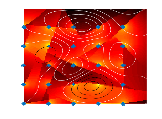
Following is the resulting timing, and Figure 2 shows a heat map showing the signal strength at each point on the map.
Signal strength compute time per gridpoint after vectorization = 0.013176ms
Speedup of 2844.3662x
Advanced vectorization
Vectorizing is advisable for any performance-critical MATLAB code, whether it uses the GPU or not. MATLAB’s documentation provides a wealth of advice on the different techniques to use, most of which apply equally well to GPU code. The trickiest scenario tends to be when the data is divided into groups or categories of different sizes since they can’t easily be given their own row, column or page of an array. gpuArray supports a number of the features that can help with this including linear and logical indexing, find, sort and accumarray.
Say we refine our example so that each antenna belongs to one of three networks and we want a signal map for each one. I can use sort to group all the signal strengths by network, diff and find to identify the boundaries between groups, and cumsum to get the average of the strongest three signals. Here’s the resulting code.
% This script divides the antennae between 3 networks
% and computes a signal map for each one independently. While this could
% be done using a loop, we prefer to use vectorized operations to process
% all the data together.

% Assign network 1-3 (at random) to each antenna at every point
Network = gpuArray.randi(3, 1, M);
NetworkReplicated = repmat(Network, [N 1]);

% Sort power data and networks by power
[signalPowerSorted, I] = sort(signalPowerDecibels, 2, 'descend');
NetworkSorted = NetworkReplicated(sub2ind([N M], RowIndex(:), I(:)));

% Sort again to group by network
[~, J] = sort(reshape(NetworkSorted, [N M]), 2);
signalPowerGrouped = signalPowerSorted(J);

% Sorting original list and diff finds group boundaries as an index array
NetworkGrouped = sort(Network);
groupStartColumn = find(diff([0, NetworkGrouped]));

% Accumulated sum will allow us to find means without loops
signalPowerCum = cumsum([zeros(N,1), signalPowerGrouped], 2);

% Pick out the sum of the three most powerful antennae to get the mean
signalMap = (signalPowerCum(:,groupStartColumn+3) - ...
             signalPowerCum(:,groupStartColumn)) / 3;
drawMultipleSignalMaps(map, masts, AntennaDirection, H, signalMap)
The complete code is available on Github.
Batching matrix operations using pagefun
Many 2-D matrix operations such as multiply and transpose do not naturally vectorize, and this can be a bottleneck when you have a large number of small matrices to operate on. pagefun provides the solution, letting you carry out a large batch of these operations in a single call.
Say I want to rotate all the antenna masts by a different horizontal (pan) and vertical (tilt) rotation. Vectorization cannot solve this problem, so I might revert to using a loop to apply the 3 x 3 rotations that make up each ‘slice’ of the 3-D Pan and Tilt arrays:
% Loop over the antennae applying the Pan and Tilt rotations defined
% earlier
newAntennaDirection = gpuArray.zeros(size(AntennaDirection));
for a = 1:M
    thisMast = AntennaDirection(:,a);
    newAntennaDirection(:,a) = Pan(:,:,a) * Tilt(:,:,a) * thisMast;
end
Time to rotate antennae using a loop = 7.885ms
Translating this into pagefun operations gives a considerable speedup even though there are only 25 simultaneous multiplies in this case.
oldDirection = reshape(AntennaDirection, [3 1 M]); % M pages of 3x1 vecs
newAntennaDirection = pagefun(@mtimes, Tilt, oldDirection);
newAntennaDirection = pagefun(@mtimes, Pan, newAntennaDirection);
Time to rotate antennae using pagefun = 0.438ms
Speedup of 18.0023x
Along with all the element-wise functions, matrix multiplication, and transpose, pagefun also supports solving small linear systems in batch using mldivide (the MATLAB backslash \ operator).
Writing kernels using arrayfun
The way that each gpuArray function is implemented varies, but typically these functions launch one or more kernels to do the bulk of the work in parallel. Kernel launches have overhead, which can add up when doing a sequence of operations on the elements of an array, such as arithmetic. For example, a calculation like
pathLoss = (4 .* pi .* distance .* Frequency ./ 3e8).^2
will launch four or five kernels, when really all the operations could be done in a single kernel.
MATLAB employs various optimizations to minimize this kind of kernel launch proliferation. However you may find you get better performance when you explicitly identify parts of your code that you know could be compiled into a single kernel. To do this, write the kernel in the MATLAB language as a function, and call it using the wrapper arrayfun. This is the last and most advanced of our wrapper family.
By splitting out the X, Y and Z coordinates, a significant portion of the power calculation can be separated into a function containing only scalar operations.
function signalPower = powerKernel(mapIndex, mastIndex)
    % Implement norm and dot product calculations via loop
    dSq = 0;
    dotProd = 0;
    for coord = 1:3
        path = A(1,mastIndex,coord) - X(mapIndex,1,coord);
        dSq = dSq + path*path;
        dotProd = dotProd + path*dirn(1,mastIndex,coord);
    end
    d = sqrt(dSq);

    % Power calculation, with adjustment for being behind antenna
    if dotProd >= 0
        pLoss = (4 .* pi .* d .* Frequency ./ 3e8).^2;
        powerWatts = Power(mastIndex) ./ pLoss;
        signalPower = 30 + 10 * log10(powerWatts);
    else
        signalPower = -inf;
    end
end
This function represents a kernel run in parallel at every data point, so one thread is run for each element of the input arrays.
signalPower = arrayfun(@powerKernel, mapIndex, mastIndex);
Like bsxfun, arrayfun takes care of expanding input arrays along dimensions that don’t match. In this case, our N x 1 map indices and our 1 x M antenna indices are expanded to give the N x M output dimensions.
Now that we’ve taken full control over the way the power calculation is parallelized, we can see a further gain over the original code:
% Original power calculation
gpuArrayTime = gputimeit(@() ...
    powerCalculationWithGpuArray(X, A, Power, Frequency, dirn) );

% Power calculation using arrayfun
arrayfunTime = gputimeit(@() ...
    arrayfun(@powerKernel, mapIndex, mastIndex) );

% Resulting performance improvement
disp(['Speedup for power calculation using arrayfun = ' ...
      num2str(gpuArrayTime/arrayfunTime) 'x']);
Speedup for power calculation using arrayfun = 2.3389x
It’s worth remarking that in order to implement versions of the vector norm and dot product inside the kernel it is necessary to use a for loop, something we were trying to avoid. However, inside the kernel this is not significant since we are already running in parallel.
arrayfun kernels support scalar functions along with the majority of standard MATLAB syntax for looping, branching, and function execution. For more detail see the documentation.
A really important feature that we’ve used here is the ability to index into arrays defined outside the nested function definition, such as A, X and Power. This simplified the kernel because we didn’t have to pass all the data in, only the indices identifying the grid reference and antenna. Indexing these upvalues works inside arrayfun kernels as long as it returns a single element.
Note that there is a one-time cost to arrayfun kernel execution while MATLAB compiles the new kernel.
Why not always write arrayfun kernels instead of writing them in another language? Well, arrayfun launches as many parallel threads as it can, but you have no control over launch configuration or access to shared memory. And of course, you cannot call into third party libraries as you could from C or C++ code. This is where CUDAKernels and MEX functions can really help.
Conclusion
Vectorization is a key concept for MATLAB programming that provides big performance advantages for both standard and GPU coding. Combining this principle with the wealth of built-in functions optimized for the GPU is usually enough to take advantage of your device, without needing to learn about CUDA or parallel programming concepts. And if that falls short, the arrayfun function lets you craft custom kernels in the MATLAB language to eke a lot more performance from your card.
Further reading
- MATLAB documentation on vectorization
- MATLAB documentation on GPU Computing
- ParallelForAll Blog article on CUDAKernels
- ParallelForAll Blog article on GPU MEX functions
- All the code needed to reproduce the examples and plots in this article is available on Github.