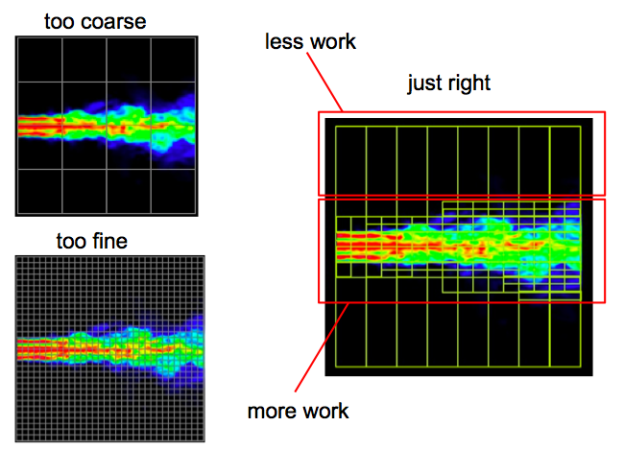
Early CUDA programs had to conform to a flat, bulk parallel programming model. Programs had to perform a sequence of kernel launches, and for best performance each kernel had to expose enough parallelism to efficiently use the GPU. For applications consisting of “parallel for” loops the bulk parallel model is not too limiting, but some parallel patterns—such as nested parallelism—cannot be expressed so easily. Nested parallelism arises naturally in many applications, such as those using adaptive grids, which are often used in real-world applications to reduce computational complexity while capturing the relevant level of detail. Flat, bulk parallel applications have to use either a fine grid, and do unwanted computations, or use a coarse grid and lose finer details.
CUDA 5.0 introduced Dynamic Parallelism, which makes it possible to launch kernels from threads running on the device; threads can launch more threads. An application can launch a coarse-grained kernel which in turn launches finer-grained kernels to do work where needed. This avoids unwanted computations while capturing all interesting details, as Figure 1 shows.
Dynamic parallelism is generally useful for problems where nested parallelism cannot be avoided. This includes, but is not limited to, the following classes of algorithms:
- algorithms using hierarchical data structures, such as adaptive grids;
- algorithms using recursion, where each level of recursion has parallelism, such as quicksort;
- algorithms where work is naturally split into independent batches, where each batch involves complex parallel processing but cannot fully use a single GPU.
Dynamic parallelism is available in CUDA 5.0 and later on devices of Compute Capability 3.5 or higher (sm_35). (See NVIDIA GPU Compute Capabilities.)
This post introduces Dynamic Parallelism by example using a fast hierarchical algorithm for computing images of the Mandelbrot set. This is the first of a three part series on CUDA Dynamic Parallelism:
- Adaptive Parallel Computation – Dynamic Parallelism overview and example (this post);
- API and Principles – Advanced topics in Dynamic Parallelism, including device-side streams and synchronization;
- Case Study: PANDA – how Dynamic Parallelism made it easier and more efficient to implement Triplet Finder, an online track reconstruction algorithm for the high-energy physics PANDA experiment, which is part of the Facility for Antiproton and Ion Research in Europe (FAIR).
Case Study: The Mandelbrot Set
The Mandelbrot set is perhaps the best known fractal. It is defined as


The interior of Figure 2 (the black part), is the Mandelbrot Set.

The Escape Time Algorithm
The most common algorithm used to compute the Mandelbrot set is the “escape time algorithm”. For each pixel in the image, the escape time algorithm computes the value dwell, which is the number of iterations it takes to decide whether the point belongs to the set. In each iteration (up to a predefined maximum), the algorithm modifies the point according to the Mandelbrot set equations and checked to see whether it “escapes” outside a circle of radius 2 centered at point (0, 0). We compute the dwell for a single pixel using the following code.
#define MAX_DWELL 512
// w, h --- width and hight of the image, in pixels
// cmin, cmax --- coordinates of bottom-left and top-right image corners
// x, y --- coordinates of the pixel
__host__ __device__ int pixel_dwell(int w, int h,
                                    complex cmin, complex cmax,
                                    int x, int y) {
  complex dc = cmax - cmin;
  float fx = (float)x / w, fy = (float)y / h;
  complex c = cmin + complex(fx * dc.re, fy * dc.im);
  complex z = c;
  int dwell = 0;

  while(dwell < MAX_DWELL && abs2(z) < 2 * 2) {
    z = z * z + c;
    dwell++;
  }

  return dwell;
}
The value of dwell determines whether the point is in the set.
- If
dwellequalsMAX_DWELL, the point belongs to the set, and is usually colored black. - If
dwellis less thanMAX_DWELL, the point does not belong to the set. We use thedwellvalue to color the pixel.
If the point does not belong to the set, lower dwell values correspond to darker colors. Generally, the nearer the point is to the Mandelbrot set, the higher its value of dwell. This is why in most Mandelbrot set images the region immediately outside the set is bright, as in Figure 2.
A Per-Pixel Mandelbrot Set Kernel
A straightforward way to compute Mandelbrot set images on the GPU uses a kernel in which each thread computes the dwell of its pixel, and then colors each pixel according to its dwell. For simplicity, we omit the coloring code, and concentrate on computing dwell in the following kernel code.
// kernel
__global__ void mandelbrot_k(int *dwells,
                             int w, int h,
                             complex cmin, complex cmax) {
  int x = threadIdx.x + blockDim.x * blockIdx.x;
  int y = threadIdx.y + blockDim.y * blockIdx.y;
  if(x < w && y < h)
    dwells[y * w + x] = pixel_dwell(w, h, cmin, cmax, x, y);
}

int main(void) {

  // ... details omitted ...

  // kernel launch
  int w = 4096, h = 4096;
  dim3 bs(64, 4), grid(divup(w, bs.x), divup(h, bs.y));
  mandelbrot_k <<<grid, bs>>>(d_dwells, w, h,
                              complex(-1.5, 1), complex(0.5, 1));

  // ...
}
This kernel runs quickly on the GPU; it can compute a 4096×4096 image with MAX_DWELL of 512 in just over 40 ms on an NVIDIA Kepler K20X accelerator. However, under closer examination, we can see that such an algorithm wastes a lot of computational resources. There are large regions inside the set that could simply be colored black; note that since MAX_DWELL iterations are performed for every black pixel, this is where the algorithm spends most of the computation time. There are also large regions of constant but low dwell outside the Mandelbrot set. In general, the only areas where we need high-resolution computation are along the fractal boundary of the set.
The Mariani-Silver Algorithm
We can exploit the large regions of uniform dwell using the hierarchical Mariani-Silver algorithm to focus computation where it is most needed. This algorithm relies on the fact that the Mandelbrot set is connected: there is a path between any two points belonging to the set. Thus, if there is a region (of any shape) whose border is completely within the Mandelbrot set, the entire region belongs to the Mandelbrot set. More generally, if the border of the region has a certain constant dwell, then every pixel in the region has the same dwell. So, if dwell is uniform, it is enough to evaluate it on the border, saving computation.
The Mariani-Silver algorithm combines this principle with recursive subdivision of regions with non-constant dwell, as described by the following pseudocode, and shown in Figure 3.
mariani_silver(rectangle)
  if (border(rectangle) has common dwell)
        fill rectangle with common dwell
    else if (rectangle size < threshold)
      per-pixel evaluation of the rectangle
    else
      for each sub_rectangle in subdivide(rectangle)
          mariani_silver(sub_rectangle)

This algorithm is a great fit for implementation with CUDA Dynamic Parallelism. Each call to the mariani_silver pseudocode routine maps to one thread block of the mandelbrot_block_k kernel. The threads of the block use a parallel reduction to determine whether border pixels all have the same dwell. Provided that we launch enough thread blocks initially, this won’t decrease the amount of parallelism available to the GPU. Thread zero in each block then decides whether to fill the region, further subdivide it, or to evaluate the dwell for every pixel of the rectangle.
Dynamic Parallelism Basics
In order to implement the Mariani-Silver algorithm with Dynamic Parallelism, we need to launch kernels from threads running on the device. This is simple because device-side kernel launches use the same syntax as launches from the host. As on the host, device kernel launch is asynchronous, meaning that control returns to the launching thread immediately after launch, (likely) before the kernel finishes. Successful execution of a kernel launch merely means that the kernel is queued; it may begin executing immediately, or it may execute later when resources become available.
Dynamic Parallelism uses the CUDA Device Runtime library (cudadevrt), a subset of CUDA Runtime API callable from device code. As on the host, all API functions return an error code, and the same best practice applies: check for errors after each API call. On CUDA versions before 6.0, device-side kernel launches may fail due to the kernel launch queue being full. So it’s very important to check for errors after each kernel launch.
To avoid writing lots of boilerplate code, we use the following macro to check errors. It checks the return code of a CUDA call, and, if an error has occurred, it prints the error code and location and terminates the kernel. The information printed is useful for debugging (See How to Query Device Properties and Handle Errors in CUDA C/C++).
#define cucheck_dev(call)                                   \
{                                                           \
  cudaError_t cucheck_err = (call);                         \
  if(cucheck_err != cudaSuccess) {                          \
    const char *err_str = cudaGetErrorString(cucheck_err);  \
    printf("%s (%d): %s\n", __FILE__, __LINE__, err_str);   \
    assert(0);                                              \
  }                                                         \
}
We wrap device CUDA calls with cucheck_err as in the following example.
cucheck_dev(cudaGetLastError());
Implementing the Mariani-Silver Algorithm with Dynamic Parallelism
Now that we know how to launch kernels and check errors in device code, we can implement the Mariani-Silver with Dynamic Parallelism. We use the following comparison code in a parallel reduction to determine whether border pixels have the same dwell.
#define NEUT_DWELL (MAX_DWELL + 1)
#define DIFF_DWELL (-1)

__device__ int same_dwell(int d1, int d2) {
  if (d1 == d2)
    return d1;
  else if (d1 == NEUT_DWELL || d2 == NEUT_DWELL)
    return min(d1, d2);
  else
    return DIFF_DWELL;
}
The following kernel implements the Mariani-Silver algorithm with Dynamic Parallelism.
#define MAX_DWELL 512
/** block size along x and y direction */
#define BSX 64
#define BSY 4
/** maximum recursion depth */
#define MAX_DEPTH 4
/** size below which we should call the per-pixel kernel */
#define MIN_SIZE 32
/** subdivision factor along each axis */
#define SUBDIV 4
/** subdivision factor when launched from the host */
#define INIT_SUBDIV 32

__global__ void mandelbrot_block_k(int *dwells,
                                   int w, int h,
                                   complex cmin, complex cmax,
                                   int x0, int y0,
                                   int d, int depth) {

  x0 += d * blockIdx.x, y0 += d * blockIdx.y;
  int common_dwell = border_dwell(w, h, cmin, cmax, x0, y0, d);
  if (threadIdx.x == 0 && threadIdx.y == 0) {
    if (common_dwell != DIFF_DWELL) {
      // uniform dwell, just fill
      dim3 bs(BSX, BSY), grid(divup(d, BSX), divup(d, BSY));
      dwell_fill<<<grid, bs>>>(dwells, w, x0, y0, d, comm_dwell);
    } else if (depth + 1 < MAX_DEPTH && d / SUBDIV > MIN_SIZE) {
      // subdivide recursively
      dim3 bs(blockDim.x, blockDim.y), grid(SUBDIV, SUBDIV);
      mandelbrot_block_k<<<grid, bs>>>
        (dwells, w, h, cmin, cmax, x0, y0, d / SUBDIV, depth+1);
    } else {
      // leaf, per-pixel kernel
      dim3 bs(BSX, BSY), grid(divup(d, BSX), divup(d, BSY));
      mandelbrot_pixel_k<<<grid, bs>>>
        (dwells, w, h, cmin, cmax, x0, y0, d);
    }
    cucheck_dev(cudaGetLastError());
  }
}  // mandelbrot_block_k

int main(void) {

  // ... details omitted ...

  // launch the kernel from the host
  int width = 8192, height = 8192;
  mandelbrot_block_k<<<dim3(init_subdiv, init_subdiv), dim3(bsx, bsy)>>>
    (dwells, width, height,
     complex(-1.5, -1), complex(0.5, 1), 0, 0, width / INIT_SUBDIV);

  // ...
}
mandelbrot_block_k kernel uses the following functions and kernels.
border_dwell: a function to check whether thedwellvalue is the same along the border of the current region; it performs a parallel reduction within a thread block.dwell_fill: sets each pixel within the given image rectangle to the specifieddwellvaluemandelbrot_pixel_k: the same per-pixel kernel we used for our first implementation, but applied only within a specific image rectangle.
The complete code for these kernels and full code for rendering the Mandelbrot set image using the Mariani-Silver algorithm is available on Github.
Compiling and Linking
To use Dynamic parallelism, you must compile your device code for Compute Capability 3.5 or higher, and link against the cudadevrt library. You must use a two-step separate compilation and linking process: first, compile your source into an object file, and then link the object file against the CUDA Device Runtime. (See Separate Compilation and Linking of CUDA C++ Device Code.)
To compile your source code into an object file, you need to specify the -c (--compile) option, and you need to specify -rdc=true (--relocatable-device-code=true) to generate relocatable device code, required for later linking. You can shorten this to -dc (--device -c), which is equivalent to combining the two options above.
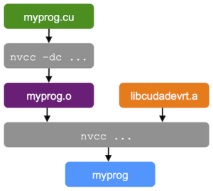
nvcc -arch=sm_35 -dc myprog.cu -o myprog.o
To link the object file with a library, use the -l option with the library, in our case, -lcudadevrt.
nvcc -arch=sm_35 myprog.o -lcudadevrt -o myprog
Figure 4 illustrates the compilation process.
Note that the -rdc=true option is not necessary in this case, because nvcc generates an executable that does not need any further linking. You can also compile and link in a single step, in which case you should specify the -rdc=true option.
nvcc -arch=sm_35 -rdc=true myprog.cu -lcudadevrt -o myprog.o
Conclusion: Higher Efficiency and Performance
Figure 5 compares the performance of the brute force per-pixel and Mariani-Silver algorithms for generating the Mandelbrot set when run on an NVIDIA Kepler K20X GPU at standard application clocks.
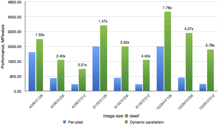
Using dynamic parallelism always leads to a performance improvement in this application. The speed up is higher at higher resolutions and higher MAX_DWELL. This makes sense, because larger MAX_DWELL means more computations we can avoid at each pixel, and higher resolution means larger regions, in terms of pixel count, where we can avoid computations. The overall speedup from using dynamic parallelism varies from 1.3x to almost 6x.
Also note that using dynamic parallelism decreases the cost of increasing MAX_DWELL to improve the accuracy of the image. While the performance of the per-pixel version drops by 6x when increasing dwell from 128 to 512, the drop is only 2x for the Dynamic Parallelism algorithm.
Using a hierarchical adaptive algorithm with Dynamic Parallelism to compute the Mandelbrot set image results in a significant performance improvement compared to a straightforward per-pixel algorithm. You can use Dynamic Parallelism in a similar way to accelerate any adaptive algorithm, such as solvers with adaptive grids.
We’ll continue this series soon with a look at more advanced Dynamic Parallelism principles, such as synchronization and device-side streams, before concluding with a real-world case study study in the third part of this series.