Note: This is the final part of a detailed three-part series on machine translation with neural networks by Kyunghyun Cho. You may enjoy part 1 and part 2.
In the previous post in this series, I introduced a simple encoder-decoder model for machine translation. This simple encoder-decoder model is excellent at English-French translation. However, in this post I will briefly discuss the weakness of this simple approach, and describe a recently proposed way of incorporating a soft attention mechanism to overcome the weakness and significantly improve the translation quality.
Furthermore, I will present some more recent works that utilize this neural machine translation approach to go beyond machine translation of text, such as image caption generation and video description generation. I’ll finish the blog series with a brief discussion of future research directions and a pointer to the open source code implementing these neural machine translation models.
The Trouble with Simple Encoder-Decoder Architectures
In the encoder-decoder architecture, the encoder compresses the input sequence as a fixed-size vector from which the decoder needs to generate a full translation. In other words, the fixed-size vector, which I’ll call a context vector, must contain every single detail of the source sentence. Intuitively, this means that the true function approximated by the encoder has to be extremely nonlinear and complicated. Furthermore, the dimensionality of the context vector must be large enough that a sentence of any length can be compressed.
In my paper “On the Properties of Neural Machine Translation: Encoder-Decoder Approaches” presented at SSST-8, my coauthors and I empirically confirmed that translation quality dramatically degrades as the length of the source sentence increases when the encoder-decoder model size is small. Together with a much better result from Sutskever et al. (2014), using the same type of encoder-decoder architecture, this suggests that the representational power of the encoder needed to be large, which often means that the model must be large, in order to cope with long sentences (see Figure 1).
Of course, a larger model implies higher computation and memory requirements. The use of advanced GPUs, such as NVIDIA Titan X, indeed helps with computation, but not with memory (at least not yet). The size of onboard memory is often limited to several Gigabytes, and this imposes a serious limitation on the size of the model. (Note: it’s possible to overcome this issue by using multiple GPUs while distributing a single model across those GPUs, as shown by Sutskever et al. (2014). However, let’s assume for now that we have access to a single machine with a single GPU due to space, power and other physical constraints.)
Then, the question is “can we do better than the simple encoder-decoder based model?”
Soft Attention Mechanism for Neural Machine Translation
The biggest issue with the simple encoder-decoder architecture is that a sentence of any length needs to be compressed into a fixed-size vector. This is a rather peculiar approach when you consider how computers typically handle compression tasks. When you zip a file, the length of the resulting compressed file is roughly proportional to the length of the original file. (This is not quite true: the compressed size is proportional to the amount of information in the original file, not its length. However, for the sake of argument, let us assume that the length of the original file closely reflects the amount of information in the file.)
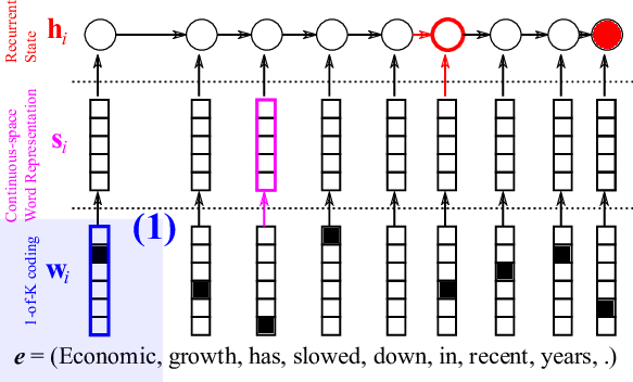
Continuing with an analogy to digital computers, let’s store the whole sentence not as a fixed-size vector, but as a memory that contains as many banks as there are source words. This is done by using a so-called bidirectional recurrent neural network (BiRNN) which consists of a forward recurrent neural network (RNN) and a separate backward RNN. As the names suggest, the forward and backward RNN’s read the source sentence in forward and backward directions, respectively.
Now, let’s call the hidden states from the forward RNN 


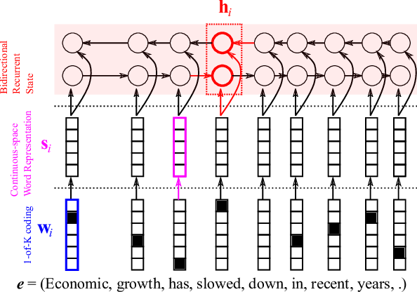
This summary at the position of each word, however, is not the perfect summary of the whole input sentence. Due to its sequential nature, a recurrent neural network tends to remember recent symbols better. In other words, the further away an input symbol is from 
This is definitely not an agreed convention, but personally, because of this reason, I understand the annotation vector as a context-dependent word representation. Furthermore, we can consider this set of context-dependent word representations as a mechanism by which we store the source sentence as a variable-length representation, as opposed to the fixed-length, fixed-dimensional summary from the simple encoder-decoder model.
With this variable-length representation of a source sentence, the decoder now needs to be able to selectively focus on one or more of the context-dependent word representations, or the annotation vectors, for each target word. So, which annotation vector should the decoder focus on each time?
Let’s imagine you’re translating the given source sentence, and you have written the first 


A typical translator looks at each source word 


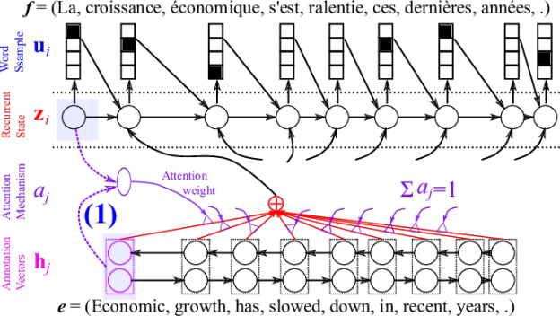
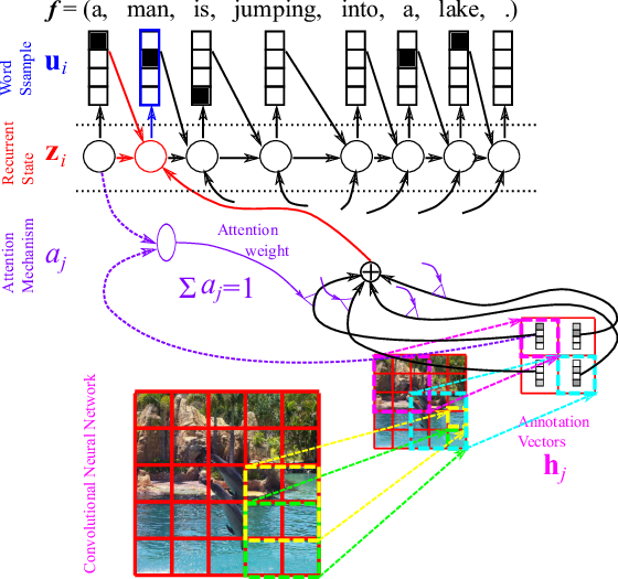
Dzmitry Bahdanau and I together with Yoshua Bengio last summer (2014) proposed to include a small neural network in a decoder to do almost exactly this. The small neural network, which we call the attention mechanism (purple-colored part in Figure 3), takes as input the previous decoder’s hidden state 

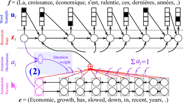
Once we’ve computed the relevance score of every source word, we want to make sure that they sum to one. This can be done easily using softmax normalization such that

See Figure 5 for the graphical illustration.
Why do we want this kind of normalization? There can be many reasons, but my favourite reason is that this helps us interpret the scores assigned by the attention mechanism in a probabilistic framework. From this probabilistic perspective, one can think of the attention weight 

![c_i = \sum_{j=1}^T \alpha_j h_j = \mathbb{E}_{\alpha_j'} \left[ h_j \right].](https://s0.wp.com/latex.php?latex=c_i+%3D+%5Csum_%7Bj%3D1%7D%5ET+%5Calpha_j+h_j+%3D+%5Cmathbb%7BE%7D_%7B%5Calpha_j%27%7D+%5Cleft%5B+h_j+%5Cright%5D.&bg=transparent&fg=000&s=0&c=20201002)
This expected vector 
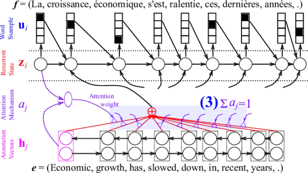
Once this vector 
What does Soft Attention Mechanism Bring to the Table?
This approach of incorporating attention mechanism has become one of the hottest topics in deep learning recently (see Cho et al., 2015 and references therein.) It would be super interesting to talk about the consequences of having attention mechanism in a neural network and how it can lead us to yet another level of success in deep learning, but that would take much more than a blog post. Instead, Figure 6 shows an example of the kind of attention (or alignment) that the model learns without any supervision on the alignment. (Note: although the term weakly supervised is often used to denote reinforcement learning, I find this type of model equally weakly supervised. Except for the final target translation, there was absolutely no supervision on the internal correspondence/attention/alignment.)
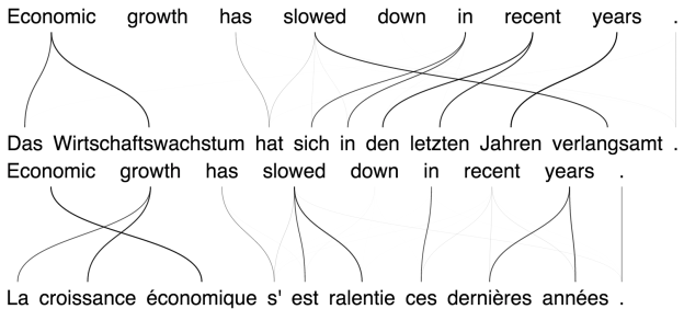
It’s pretty awesome that the model automatically found the correspondence structure between two languages. I’m sure you’ll appreciate it better if you speak either French or German (both of which I don’t)! But, the bigger question is, does the introduction of the attention mechanism improve translation performance?
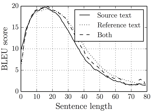
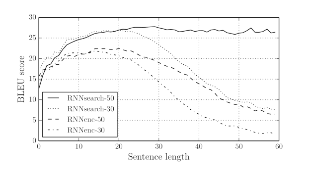
Yes, it does, and quite tremendously! Especially, in [Bahdandau et al., 2015], we observed that with the addition of the attention mechanism, the quality of the translation does not drop as sentence length increases, even when the size of the model stays roughly the same, as Figure 7 shows.
The last issue is that this looks way too complicated to implement. Again, Theano to the rescue! Just write a forward computation pass (see here for an example) and use theano.tensor.grad, and you’re ready to go.
Neural Turing Machines and Memory Networks
Reader Zzzz commented on my previous post in this series:
Have you guys tried to use Neural Turing Machine or memory networks for this purpose? Or those models require much bigger training sets to produce better results?
I meant to write a response sooner, but decided to wait until this post. Why? Because, both the neural Turing machine (NTM) by Graves et al. (2014) as well as the memory networks by Weston et al. (2014) can be thought of as variants/extensions of the described neural machine translation with soft attention mechanism. Think of the set of context-dependent word representations
In fact, if you read the latest paper on memory networks by Sukhbaatar et al. (2015), it becomes very clear that the attention-based neural machine translation, the NTM and the memory networks are more or less equivalent except for some details and for which applications they were designed. I, and probably you as well, have to wonder what will be the ultimate generalization of all these approaches and what kind of consequences this ultimate model will bring in the future.
Beyond translation: Image/Video Caption Generation
The most surprising and important point of this whole neural machine translation business is that there’s nothing specific to languages. In particular, this approach can handle any type of input data as long as there’s a suitable neural architecture that returns either a fixed-size vector representation of the input or a set of annotation vectors of it.
A recently published work from the University of Montreal and the University of Toronto showed that it is possible to design an attention-based encoder-decoder model which describes an image by replacing the encoder with a convolutional neural network, as Figure 8 shows. Similar approaches were proposed also in [Donahue et al., 2014; Fang et al., 2014; Karpathy and Li, 2014; Kiros et al., 2014; Mao et al., 2014].

Pushing the boundary further, Li et al. (2015) applied a similar attention-based approach to video description generation by letting the decoder utilize temporal structures of the video. Similarly, video description generation with the simple encoder-decoder architecture was proposed recently by [Li et al., 2015; Venugopalan et al., 2015] (See Figure 9).
![Figure 9. Temporal attention for video description generation. From [Li et al., 2015].](/blog/wp-content/uploads/2015/07/Figure9_video_description-624x382.png)
Looking at all these recent works makes me wonder what will come next. What do you think? Let me know in the comments to this post.
What’s Next?
In this post, I introduced recent advances in deep learning, centered around neural machine translation. However, there are many challenges related to neural machine translation remaining to be solved in the future. Let me list a few of them here.
- Beyond modeling sentences: Sentences, when represented as a sequence of words, are very short. The backpropagation algorithm for recurrent neural networks requires time proportional to the length of a sequence. Can there be another algorithm more suitable for dealing with much longer sequences, such as paragraphs and documents? Learning should probably be local, and weights should be updated online while processing a sequence.
- Beyond natural languages: Neural machine translation works for languages, but what else can it work for? Perhaps gene expression sequences, protein structure prediction, graphs and social networks, or weather data?
- Multimodal learning: Can we leverage other sources of information for translation? What is the natural way to incorporate multiple sources of information?
Where’s the Code?
In this series so far I have avoided the discussion on the practical implementation. However, we at the University of Montreal have been actively making our code publicly available, because we believe open-source code helps speed up research progress by letting everyone try the code and easily customize or build upon it.
One of the most important contributions we have made in recent years has been Theano. Theano is a tool specialized in symbolically building an arbitrary neural network using Python. It abstracts the underlying compute architecture such that the same code can be run either on a more traditional CPU-based backend or on a more specialized hardware architecture such as GPUs. Furthermore, Theano implements symbolic differentiation which is crucial in training a neural network, making it extremely simple to quickly prototype complicated neural networks (such as the attention-based neural machine translation model described in this post). However, Theano only provides basic primitives, and one needs to sew those primitives into a neural network, which is not at all a trivial task even with Theano.
We (Razvan Pascanu, Caglar Gulcehre, myself, Dzmitry Bahdanau and Bart van Merrienboer) earlier released GroundHog which implements all the necessary components to build a neural machine translation model. Unfortunately, this code was rather hastily developed, and the readability is extremely low. Since then, Orhan Firat, Dzmitry Bahadanu and Bart van Merrienboer prepared an example script to build, train and use neural machine translation models based on the newly introduced framework called Blocks. However, this should also be treated only as an example for now.
In October this year (2015) at Dublin City University I will give a lecture on neural machine translation as part of the DL4MT Winter School. To make the winter school more useful and practical for the audience, I am now preparing a stripped-down version of neural machine translation based on Theano. The code, which is called dl4mt-material and still in heavy preparation, can be found here.
Currently, this code includes three subdirectories; session0, session1 and session2. session0 contains the implementation of the recurrent neural network language model using gated recurrent units, and session1 the implementation of the simple neural machine translation model. In session2, you can find the implementation of the attention-based neural machine translation model we discussed today. I am planning to make a couple more sessions, so stay tuned!
Oh, one more thing before I finish this section, and the whole series. Let me make it clear again: always train this type of model with GPUs! To get a well-trained model, it takes about three to twelve days using a GeForce GTX Titan X, and with CPUs, I cannot even give any reasonable estimate on how long it will take to train a model. Of course, you can probably build a Google-sized cluster and use a distributed optimization algorithm, but I believe this is probably not the most cost-efficient way to go (unless you’re Microsoft, Facebook or IBM).
Acknowledgements
I’ve covered a lot of recent research in this series of Parallel Forall posts on Neural Machine Translation. Hopefully I didn’t make it sound like I did all this work on my own. Any work introduced here has been done by all the authors in the cited papers including those at the University of Montreal as well as other institutes. Furthermore, most of my work in the past few years wouldn’t have been possible without the availability of Theano, and I’d like to thank all the contributors to Theano, and especially, Fred Bastien, Pascal Lamblin and Arnaud Bergeron.
Note that any error in the text is my own, and feel free to contact me if you found anything suspicious here.
References
- Bahdanau, Dzmitry, Kyunghyun Cho, and Yoshua Bengio. “Neural machine translation by jointly learning to align and translate.” arXiv preprint arXiv:1409.0473 (2014).
- Bastien, Frédéric et al. “Theano: new features and speed improvements.” arXiv preprint arXiv:1211.5590 (2012).
- Bergstra, James et al. “Theano: a CPU and GPU math expression compiler.” Proceedings of the Python for scientific computing conference (SciPy) 30 Jun. 2010: 3.
- Bridle, J. S. (1990). Training Stochastic Model Recognition Algorithms as Networks can lead to Maximum Mutual Information Estimation of Parameters. In Touretzky, D., editor, Advances in Neural Information Processing Systems, volume 2, (Denver, 1989).
- Brown, Peter F et al. “The mathematics of statistical machine translation: Parameter estimation.” Computational linguistics 19.2 (1993): 263-311.
- Cho, Kyunghyun et al. “Learning phrase representations using RNN encoder-decoder for statistical machine translation.” arXiv preprint arXiv:1406.1078 (2014).
- Cho, Kyunghyun, Aaron Courville, and Yoshua Bengio. “Describing Multimedia Content using Attention-based Encoder–Decoder Networks.” arXiv preprint arXiv:1507.01053 (2015).
- Denil, Misha et al. “Learning where to attend with deep architectures for image tracking.” Neural computation 24.8 (2012): 2151-2184.
- Donahue, Jeff et al. “Long-term recurrent convolutional networks for visual recognition and description.” arXiv preprint arXiv:1411.4389 (2014).
- Fang, Hao et al. “From captions to visual concepts and back.” arXiv preprint arXiv:1411.4952 (2014).
- Forcada, Mikel L, and Ñeco, Ramón P. “Recursive hetero-associative memories for translation.” Biological and Artificial Computation: From Neuroscience to Technology (1997): 453-462.
- Graves, Alex, Greg Wayne, and Ivo Danihelka. “Neural Turing Machines.” arXiv preprint arXiv:1410.5401 (2014).
- Graves, Alex, Greg Wayne, and Ivo Danihelka. “Neural Turing Machines.” arXiv preprint arXiv:1410.5401 (2014).
- Gregor, Karol et al. “DRAW: A recurrent neural network for image generation.” arXiv preprint arXiv:1502.04623 (2015).
- Gulcehre, Caglar et al. “On Using Monolingual Corpora in Neural Machine Translation.” arXiv preprint arXiv:1503.03535 (2015).
- Kalchbrenner, Nal, and Phil Blunsom. “Recurrent Continuous Translation Models.” EMNLP 2013: 1700-1709.
- Karpathy, Andrej, and Li, Fei-Fei. “Deep visual-semantic alignments for generating image descriptions.” arXiv preprint arXiv:1412.2306 (2014).
- Kingma, D. P., and Ba, J. “A Method for Stochastic Optimization.” arXiv preprint arXiv:1412.6980 (2014).
- Kiros, Ryan, Ruslan Salakhutdinov, and Richard S Zemel. “Unifying visual-semantic embeddings with multimodal neural language models.” arXiv preprint arXiv:1411.2539 (2014).
- Koehn, Philipp. Statistical machine translation. Cambridge University Press, 2009.
- Mao, Junhua et al. “Deep Captioning with Multimodal Recurrent Neural Networks (m-RNN).” arXiv preprint arXiv:1412.6632 (2014).
- Mnih, Volodymyr, Nicolas Heess, and Alex Graves. “Recurrent models of visual attention.” Advances in Neural Information Processing Systems 2014: 2204-2212.
- Pascanu, Razvan et al. “How to construct deep recurrent neural networks.” arXiv preprint arXiv:1312.6026 (2013).
- Schwenk, Holger. “Continuous space language models.” Computer Speech & Language 21.3 (2007): 492-518.
- Sukhbaatar, Sainbayar et al. “End-To-End Memory Networks.”
- Sutskever, Ilya, Oriol Vinyals, and Quoc V. Le. “Sequence to sequence learning with neural networks.” Advances in Neural Information Processing Systems 2014: 3104-3112.
- Venugopalan, Subhashini et al. “Sequence to Sequence–Video to Text.” arXiv preprint arXiv:1505.00487 (2015).
- Weston, Jason, Sumit Chopra, and Antoine Bordes. “Memory networks.” arXiv preprint arXiv:1410.3916 (2014).
- Xu, Kelvin et al. “Show, Attend and Tell: Neural Image Caption Generation with Visual Attention.” arXiv preprint arXiv:1502.03044 (2015).
- Yao, Li et al. “Video description generation incorporating spatio-temporal features and a soft-attention mechanism.” arXiv preprint arXiv:1502.08029 (2015).
- Zeiler, Matthew D. “ADADELTA: an adaptive learning rate method.” arXiv preprint arXiv:1212.5701 (2012).

![Figure 3. Graphical illustration of different types of recurrent neural networks. From [Pascanu et al., 2014]](https://developer-blogs.nvidia.com/wp-content/uploads/2015/05/Figure_3.png)