![Figure 3. Graphical illustration of different types of recurrent neural networks. From [Pascanu et al., 2014]](https://developer-blogs.nvidia.com/wp-content/uploads/2015/05/Figure_3.png)
Note: This is the first part of a detailed three-part series on machine translation with neural networks by Kyunghyun Cho. You may enjoy part 2 and part 3.
Neural machine translation is a recently proposed framework for machine translation based purely on neural networks. This post is the first of a series in which I will explain a simple encoder-decoder model for building a neural machine translation system [Cho et al., 2014; Sutskever et al., 2014; Kalchbrenner and Blunsom, 2013]. In a later post I will describe how an attention mechanism can be incorporated into the simple encoder-decoder model [Bahdanau et al., 2015], leading to the state-of-the-art machine translation model for a number of language pairs including En-Fr, En-De, En-Tr and En-Zh [Gulcehre et al., 2015; Jean et al., 2015]. Furthermore, I will introduce recent work which has applied this framework of neural machine translation to image and video description generation [Xu et al., 2015; Li et al., 2015].
Statistical Machine Translation
First, let’s start with a brief overview of machine translation. In fact, the name, machine translation, says everything. We want a machine to translate text in one language, which we will call the source sentence, to corresponding text in another language, which we call the target sentence. (Although ideally the machine should be able to translate a whole document from one language to another, let us concentrate in this blog post on sentence-level machine translation.)
There are multiple ways to build such a machine that can translate languages. For instance, we can ask a bilingual speaker to give us a set of rules transforming a source sentence into a correct translation. This is not a great solution, as you can imagine, because we don’t even know the set of rules underlying a single language, not to mention the rules underlying a pair of languages. It is simply hopeless to write an exhaustive set of rules for translating a source sentence into a correct translation. Hence, in this blog post, we focus on a statistical approach where those rules, either implicitly or explicitly, are automatically extracted from a large corpus of text.
This statistical approach to machine translation is called statistical machine translation. The goal is the same (build a machine that translates a sentence from one language to another), but we let the machine learn from data how to translate rather than design a set of rules for the machine (See Fig. 1 for a graphical illustration.) Learning is based on statistical methods, which should sound familiar to anyone who has taken a basic course on machine learning. In fact, statistical machine translation is nothing but a particular application of machine learning, where the task is to find a function that maps from a source sentence to a corresponding target.

One important characteristics of machine translation is that the target (translation) function is neither one-to-one nor many-to-one as in many other applications of machine learning (such as classification, which is many-to-one), but one-to-many in the sense that one source sentence can be translated into many possible translations. Because of this, we model the translation function not as a deterministic function but as a conditional probability 


Now let’s say you want to build a statistical machine translation system that translates a source sentence in English to a sentence in French. The first and probably most important job is to collect pairs of source sentences and their corresponding translations. I will use 


Where can I get these training pairs? For widely used languages in machine translation, you probably want to check out the Workshop on Statistical Machine Translation or the International Workshop on Spoken Language Translation.
With the training data 


If the log-likelihood 
In machine learning, this is known as a maximum likelihood estimator. But we’re left with a perhaps more important question: how do we model 
Statistical Machine Translation (almost) from Scratch
This question of how to model the conditional distribution

where 

In this approach of statistical machine translation, often the only thing left to machine learning is to find a nice set of coefficients 
![Figure 2. Graphical illustration of Neural MT, SMT+Reranking-by-NN and SMT-NN. From [Bahadanau et al., 2015] slides at ICLR 2015.](/blog/wp-content/uploads/2015/05/smt_nmt-624x351.png)
In this blog post, on the other hand, I focus on a recently proposed approach, called neural machine translation, where machine learning, and more specifically a neural network, has more or even full control, as in the left panel of Fig. 2.
Neural Machine Translation
As is usual with general deep learning, neural machine translation (NMT) does not rely on pre-designed feature functions. (By pre-designed feature functions, I mean those that are not learned.) Rather, the goal of NMT is to design a fully trainable model of which every component is tuned based on training corpora to maximize its translation performance.
A fully trainable NMT model 

Given a source sequence 
Recurrent Neural Networks
One important property of machine translation, or any task based on natural languages, is that we deal with variable-length input 

To deal with these types of variable-length input and output, we need to use a recurrent neural network (RNN). Widely used feed-forward neural networks, such as convolutional neural networks, do not maintain internal state other than the network’s own parameters. Whenever a single sample is fed into a feed-forward neural network, the network’s internal state, or the activations of the hidden units, is computed from scratch and is not influenced by the state computed from the previous sample. On the other hand, an RNN maintains its internal state while reading a sequence of inputs, which in our case will be a sequence of words, thereby being able to process an input of any length.
Let me explain this in more detail. The main idea behind RNNs is to compress a sequence of input symbols into a fixed-dimensional vector by using recursion. Assume at step 


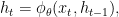
where 


![Figure 3. Graphical illustration of different types of recurrent neural networks. From [Pascanu et al., 2014]](/blog/wp-content/uploads/2015/05/Figure_3-624x208.png)
The recurrent activation function 

In this formulation, the parameters include the input weight matrix 


This simple type of RNN can be implemented very easily using (for instance) Theano, which allows your RNN to be run on either the CPU or the GPU transparently. See Recurrent Neural Networks with Word Embeddings; note that the whole RNN code is written in less than 10 lines!
Recently, it has been observed that it is better, or easier, to train a recurrent neural network with more sophisticated activation functions such as long short-term memory units [Hochreiter and Schmidhuber, 1997] and gated recurrent units [Cho et al., 2014].


As was the case with the simple recurrent activation function, the parameters here include the input weight matrices 


Although these units look much more complicated than the simple RNN, the implementation with Theano, or any other deep learning framework, such as Torch, is just as simple. For instance, see LSTM Networks for Sentiment Analysis (example code of an LSTM network).
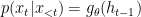
I have explained a recurrent neural network (RNN) as a history compressor, but it can also be used to probabilistically model a sequence. Here, by probabilistically modeling a sequence I mean a machine learning model that computes the probability 
Let’s start by rewriting 

which comes from the definition of conditional probability, 

Now, we let an RNN model 


There are a lot of interesting properties and characteristics of a recurrent neural network that I would love to spend hours talking about, but I will have to stop here for this blog post, since after all, what I have described so far are all the things you need to start building a neural machine translation system. For those who are more interested in recurrent neural networks, I suggest you to read the following papers. Obviously, this list is definitely not exhaustive. Or, you can also check out my slides on how to use recurrent neural networks for language modeling.
- Graves, Alex. “Generating sequences with recurrent neural networks.” arXiv preprint arXiv:1308.0850 (2013).
- Pascanu, Razvan et al. “How to construct deep recurrent neural networks.” arXiv preprint arXiv:1312.6026 (2013).
- Boulanger-Lewandowski, Nicolas, Yoshua Bengio, and Pascal Vincent. “Modeling temporal dependencies in high-dimensional sequences: Application to polyphonic music generation and transcription.” arXiv preprint arXiv:1206.6392 (2012).
- Mikolov, Tomas et al. “Recurrent neural network based language model.” INTERSPEECH 2010, 11th Annual Conference of the International Speech Communication Association, Makuhari, Chiba, Japan, September 26-30, 2010 1 Jan. 2010: 1045-1048.
- Hochreiter, Sepp, and Jürgen Schmidhuber. “Long short-term memory.” Neural computation 9.8 (1997): 1735-1780.
- Cho, Kyunghyun et al. “Learning phrase representations using rnn encoder-decoder for statistical machine translation.” arXiv preprint arXiv:1406.1078 (2014).
- Bengio, Yoshua, Patrice Simard, and Paolo Frasconi. “Learning long-term dependencies with gradient descent is difficult.” Neural Networks, IEEE Transactions on 5.2 (1994): 157-166.
The Story So Far, and What’s Next
In this post, I introduced machine translation, and described how statistical machine translation approaches the problem of machine translation. In the framework of statistical machine translation, I have discussed how neural networks can be used to improve the overall translation performance.
The goal of this blog series is to introduce a novel paradigm for neural machine translation; this post laid the groundwork, concentrating on two key capabilities of recurrent neural networks: sequence summarization and probabilistic modeling of sequences.
Based on these two properties, in the next post, I will describe the actual neural machine translation system based on recurrent neural networks. I’ll also show you why GPUs are so important for Neural Machine Translation! Stay tuned.