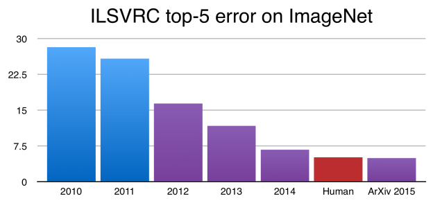
Deep learning is becoming extremely popular due to several breakthroughs in various well-known tasks in artificial intelligence. For example, at the ImageNet Large Scale Visual Recognition Challenge, the introduction of deep learning algorithms into the challenge reduced the top-5 error by 10% in 2012. Every year since then, deep learning models have dominated the challenges, significantly reducing the top-5 error rate every year (see Figure 1). In 2015, researchers have trained very deep networks (for example, the Google “inception” model has 27 layers) that surpass human performance.
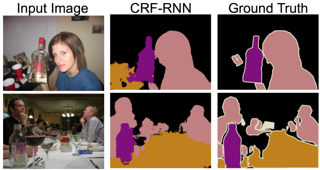
Moreover, at this year’s Computer Vision and Pattern Recognition (CVPR) conference, deep neural networks (DNNs) were being adapted to increasingly more complicated tasks. For example, in semantic segmentation, instead of predicting a single category for a whole image, a DNN is trained to classify each pixel in the image, essentially producing a semantic map indicating every object and its shape and location in the given image (see Figure 2).
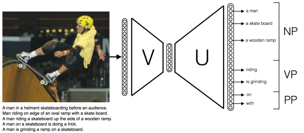
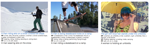
Going one step further, the relationship among those objects can be used to produce a summary of the scene. In other words, given an image, the task of image captioning is to produce a sentence describing the image. Several research groups are making promising progress on this difficult task by combining convolutional neural networks (CNNs) for computer vision and recurrent neural networks (RNNs) for natural language processing (see Figures 3 and 4).
Deep neural networks and especially RNNs are also widely applied in automatic speech recognition (ASR) systems not only in academic but also in commercial applications. Almost all of the major speech recognition services we use in our everyday life including those built by Apple, Google, Microsoft, and Baidu are all backed with industrial level deep learning.
As a final example, recently Google Deep Mind successfully applied deep learning techniques to reinforcement learning and trained models to automatically learn to play video games. They published their results in Nature and it attracted a lot of public attention because the tasks they considered here are closer to “real AI” problems.
Deep Learning Frameworks are Key
Despite outperforming the state-of-the-art in many fields, deep learning models are nothing mysterious. They are the same neural network models that have been known for decades, but with a lot more layers, trained using a huge number of training samples, and with high-performance parallel computing platforms (such as GPUs), and clever optimization techniques.
All of these factors contribute to the success of deep learning models, but one that is often under-appreciated is the separation of computation and structure (network architecture). Traditional machine learning models like Support Vector Machines (SVMs) and logistic regression models are typically presented as a holistic model. However, in deep learning, the computations are abstracted into “layers”, with the notion of forward and backward propagation. What’s important here is that the computation of each layer is completely isolated from the external world. During the forward pass, a layer takes data from a set of lower-level layers and produces the output for upper-level layers, and it does not need to know the type of the layers below or above to carry out the computation. The same thing happens in the backpropagation pass.
As a result, the implementation of deep learning models are typically separated into two parts: the framework or library, which implements various layer types as building blocks (typically with the help of highly-optimized linear algebra procedures like BLAS and GPU back-ends), and the architecture component, which is usually problem- or domain-specific. With working knowledge of a particular field, researchers are able to develop novel architectures that suit the specific problems they are interested in. The merit is they can build models that are highly efficient (which is critical for even research purpose deep models because they need to be trained on huge datasets) without needing to worry about the low-level implementation details. In other words, deep learning frameworks, in a way, provide a very high-level language for defining machine learning models.
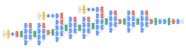
Figure 5 shows the architecture of the “Inception” deep neural network model that Google used for the ImageNet Challenge. It is a very complicated network with 27 layers with a lot of network compositions using the technique known as “Network-in-Network.” Without the easily composable computation units provided by deep learning frameworks, implementing such a huge model would be a nightmare.
Even classical shallow models become special cases under this framework. For example, SVMs are nothing more than inner-product layers trained with a hinge-loss layer, while logistic regression is just a soft-max layer on top of an inner-product layer.
Fortunately, nowadays a lot of high-quality deep learning libraries are emerging. The relatively more popular ones include Caffe from Berkeley, Torch (used by Facebook and Google DeepMind, among others), Theano from Université de Montréal and many wrappers on top of it, as well as matconvnet from the Oxford VGG group, neon from Nervana, and cxxnet.
Introducing Mocha.jl
Mocha.jl is a deep learning library for Julia, a new programming language created at MIT that is designed specifically for scientific and numerical computing. Julia is a general-purpose language with many advanced features including type inference and multiple dispatch. Moreover, Julia’s performance in benchmarks is almost comparable to C code. While still at a very young stage, Julia is becoming popular in the numerical computing world. Mocha.jl has a number of nice features and benefits, including the following.
- Written in Julia and for Julia: Mocha.jl is written in Julia, which means it has native Julia interfaces. Therefore, it is capable of interacting with core Julia functionality as well as other Julia packages.
- Minimum dependencies: to use the Julia backend, just run add(‘Mocha’) in the Julia console and the package will be installed automatically. There is no need for root privileges or installation of any external dependencies. Also, installing Julia itself is simply a matter of unpacking the archive to anywhere.
- Multiple backends: The default Julia backend is good for fast prototyping and experimenting with network architectures. If a large network is to be trained with a dataset at the scale of ImageNet, working with GPUs is necessary. Mocha.jl also comes with a GPU backend, combining customized kernels with highly efficient libraries from NVIDIA (cuBLAS, cuDNN, etc.). The GPU backend is completely compatible with Julia, and one can switch between backends by simply changing one line of code. The cuDNN-accelerated GPU backend is typically 20 or more timesfaster than the CPU-based pure Julia backend.
- Modularity and correctness: Mocha.jl is implemented in a modular architecture, making it easy to compose, customize or extend. This also makes it possible to cover all the computation units with unit tests to ensure correctness.
A Simple Mocha.jl Example
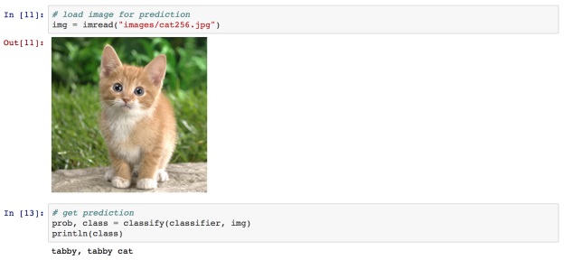
As a first example, here is a demo running a Mocha.jl deep neural network in an IJulia notebook for image classification. Specifically, we load a convolutional neural network pre-trained on the ImageNetdata, and use it to classify images.
The most important part is to construct a network by specifying a backend (CPU or GPU), and a set of layers. Then the previously trained network parameters can be loaded from a saved HDF5 file.
net = Net("imagenet", backend, layers)
h5open("model/bvlc_reference_caffenet.hdf5", "r") do h5
   load_network(h5, net)
end
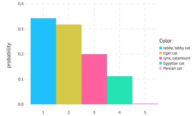
The classifier is a thin wrapper around a network that converts the numerical 1000-way prediction into the corresponding ImageNet text labels. Check out this preview of the IJulia notebook to see more details. Before proceeding to the next example, the following code shows how to use the Julia Gadfly package to make a plot of the top-5 predictions of the cat image in Figure 6. The height of each bar in the plot in Figure 7 represents the prediction confidence. As you can see, it is very easy to interact with other Julia packages.
using Gadfly

n_plot = 5
n_best = sortperm(vec(prob), rev=true)[1:n_plot]
best_probs = prob[n_best]
best_labels = classes[n_best]

plot(x=1:length(best_probs), y=best_probs, color=best_labels,
     Geom.bar, Guide.ylabel("probability"))
Fully Programmable Network Architecture Definition
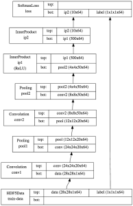
The following code demonstrates an example of defining the “LeNet” network on the MNIST handwritten digit dataset with Mocha.jl.
data_layer = AsyncHDF5DataLayer(name="train-data", source="data/train.txt", batch_size=64, shuffle=true)
 conv_layer = ConvolutionLayer(name="conv1", n_filter=20, kernel=(5,5), bottoms=[:data], tops=[:conv])
 pool_layer = PoolingLayer(name="pool1", kernel=(2,2), stride=(2,2), bottoms=[:conv], tops=[:pool])
 conv2_layer = ConvolutionLayer(name="conv2", n_filter=50, kernel=(5,5), bottoms=[:pool], tops=[:conv2])
 pool2_layer = PoolingLayer(name="pool2", kernel=(2,2), stride=(2,2), bottoms=[:conv2], tops=[:pool2])
 fc1_layer   = InnerProductLayer(name="ip1", output_dim=500, neuron=Neurons.ReLU(), bottoms=[:pool2], tops=[:ip1])
 fc2_layer   = InnerProductLayer(name="ip2", output_dim=10, bottoms=[:ip1], tops=[:ip2])
 loss_layer = SoftmaxLossLayer(name="loss", bottoms=[:ip2,:label])
As you can can see from the code, the architecture contains two convolution-pooling layers, and then two fully connected layers. Figure 8 shows how the architecture can be visualized with GraphViz by calling net2dot as in the following code.
open("net.dot", "w") do out net2dot(out, net) end
run(`dot -Tpng net.dot` |> "net.png")
Unlike many other deep neural network libraries, Mocha.jl does not use a configuration file to describe the network architecture. Instead, the layers are defined directly in Julia code. This gives us the full flexibility when experimenting with various architectures. For example, I can easily try network architecture with various layers and different nonlinearity using the following code.
hidden_layers = map(1:n_hidden_layer) do i
  InnerProductLayer(name="ip$i", output_dim=n_units_hidden,
      bottoms=[i == 1 ? :data : symbol("ip$(i-1)")],
      tops=[symbol("ip$i")],
      weight_cons=L2Cons(10),
      neuron = neuron == :relu ? Neurons.ReLU() : Neurons.Sigmoid())
end
A difference between Mocha.jl and Caffe is that nonlinearities like sigmoid or ReLU are not a separate layer. Instead, they are called “neurons”, and they can be attached to various computation layers.
The architecture of the network constructed with those layers is completely specified by connecting the “tops” (output blobs) of a layer to the “bottoms” (input blobs) to another layer, matched by the blob names. Note the layers do not need to be specified in top-to-bottom order. Mocha.jl does a topological sort of the layers and tries to verify that the network architecture is valid.
After defining the network, a stochastic gradient solver can be initialized to train the network. Mocha.jl allows full control over all the solver parameters such as the learning rate policy, the moment policy, etc. It also supports periodically inspecting the training progress and updating training parameters (e.g. halve the learning rate when the performance on a validation set decreases) via the solver’s “coffee breaks” mechanism.
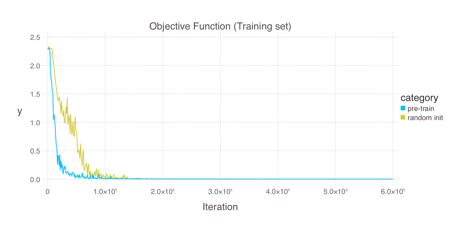
Mocha.jl can automatically save snapshots to disk during training, so you can interrupt the training process and resume it later. Also, Mocha.jl records training statistics in JLD files, which you can use to visualize the training process. For example, Figure 9 shows the learning curves of a randomly initialized deep neural network and one initialized by unsupervised pre-training using autoencoders.
To learn more about Mocha.jl, please refer to the documentation. You can also learn from the tutorials included in the documentation, the code for which is included in the “examples” directory of the Mocha.jl package.