![]() Recent advances in deep learning have enabled research and industry to master many challenges in computer vision and natural language processing that were out of reach until just a few years ago. Yet computer vision and natural language processing represent only the tip of the iceberg of what is possible. In this article, I will demonstrate how Sebastian Heinz,
Recent advances in deep learning have enabled research and industry to master many challenges in computer vision and natural language processing that were out of reach until just a few years ago. Yet computer vision and natural language processing represent only the tip of the iceberg of what is possible. In this article, I will demonstrate how Sebastian Heinz,
Roland Vollgraf and I (Calvin Seward) used deep neural networks in steering operations at Zalando’s fashion warehouses.
As Europe’s leading online fashion retailer, there are many exciting opportunities to apply the latest results from data science, statistics, and high-performance computing. Zalando’s vertically integrated business model means that I have dealt with projects as diverse as computer vision, fraud detection, recommender systems and, of course, warehouse management.
To solve the warehouse management problem that I’ll discuss in this post, we trained a neural network that very accurately estimates the length of the shortest possible route that visits a set of locations in the warehouse. I’ll demonstrate how we used this neural network to greatly accelerate a processing bottleneck, which in turn enabled us to more efficiently split work between workers.
The core idea is to use deep learning to create a fast, efficient estimator for a slow and complex algorithm. This is an idea that can (and will) be applied to problems in many areas of industry and research.
The Picker Routing Problem
For the scope of this article, we’ll restrict ourselves to a very simplified warehouse control situation in which we consider a warehouse that consists of only one zone with a “rope ladder” layout. The rope ladder layout means that items are stored in shelves, and the shelves are organized in multiple rows with aisles and cross aisles. Some of these shelves contain items that customers have ordered and must be retrieved by a worker. See Figure 1 for a schematic representation of the situation.

In 2013, we tackled the so-called “picker routing” problem: given a list of items that a worker should retrieve from the warehouse (the “pick list”), find the most efficient route or “pick tour” for the worker to walk. In a pick tour, the worker starts with an empty cart at the depot, walks through the warehouse placing items into the cart and finishes with the full cart at the depot. This is essentially a special case of the traveling salesman problem (TSP). Although the TSP is NP-hard in general, by exploiting the rope ladder layout, the optimal solution to our picker routing problem can be found in linear time in the number of aisles. The details of the exact algorithm are discussed in [1] and [2], which details an even simpler case.
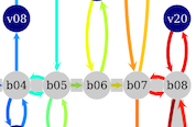
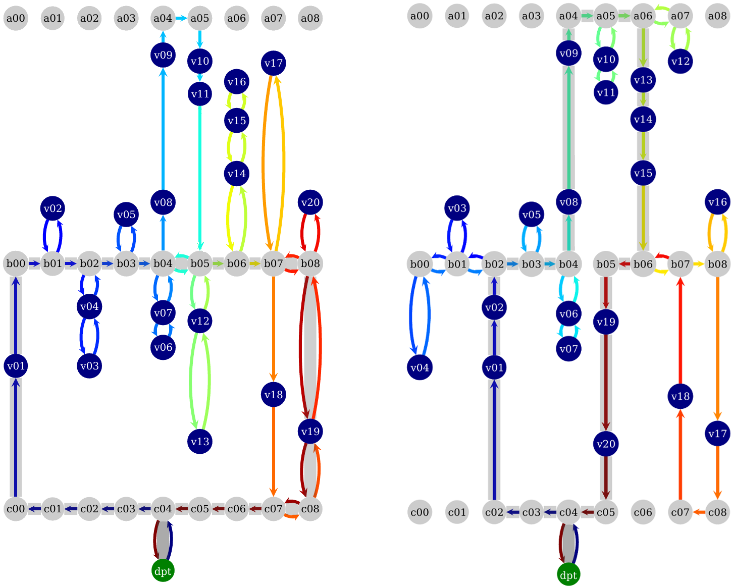
Our contribution to the problem was to come up with the OCaPi algorithm, short for Optimal Cart Pick. This algorithm finds the optimal pick tour not just for the worker, but also for the movements of the worker’s cart. A worker in the warehouse is no different from a shopper in a supermarket; the slow and heavy cart is sometimes left in the cross aisle as the worker picks until no more items can be carried. Only then does the worker return to the cart and deposit the items. A nice explanation of the project can be found here and we’ll be publishing the algorithm soon. All this enabled us to quit using the S-Shape routing heuristic [3] and route the workers and their carts optimally. See Figure 2 for an example of S-Shape and OCaPi routes.
The Batching Problem
At Zalando’s scale of operations, thousands of new orders are placed every hour, and each order must be assigned to a pick list. Only when a pick list contains a certain number of items are the items collected and packaged for the customer. For our idealized example, we assume that the following rules must be followed when splitting orders into pick lists.
- A pick list may not exceed a certain length.
- Items in an order may not be split between pick lists. In this way, all the items in an order are already together when the cart’s contents are sent to be packaged for shipping.
- The sum of the travel times (time walking plus time pushing the cart) for all pick list should be as small as possible.
For example, assume that we have 10 orders, each consisting of two items. Further assume that a worker can fit only 10 items into the cart. Then the orders must be split into two equal sized pick lists. See Figures 3 and 4 for two possible splits of the orders into pick lists. This is a highly idealized situation, [4] presents a complete picture.


In theory, finding near-optimal splits of orders into pick lists should be easy enough: just split the orders into pick lists, use the OCaPi algorithm to calculate travel times for all lists, and optimize with something like simulated annealing to find the minimum travel time split. One major problem with this idea is the OCaPi run time. At a few seconds per pick list, the OCaPi algorithm is just too slow for real world batching problems (think splitting orders between thousands of pick lists).
Neural Network OCaPi Travel Time Estimator
The OCaPi algorithm is nothing more than a very complicated highly non-linear function

Given 


From Figure 5, and by thinking about the problem it is easy to see (and can be proven) that
- Lipschitz continuous in the real-valued arguments with the Lipschitz constant equal to the worker’s walking speed;
- Piecewise linear in the real-valued arguments, with slope either flat or equal to the worker’s walking speed;
- Locally sensitive, meaning that the route a worker and cart take at a specific location is more strongly influenced by nearby items than far away items.
Therefore, since
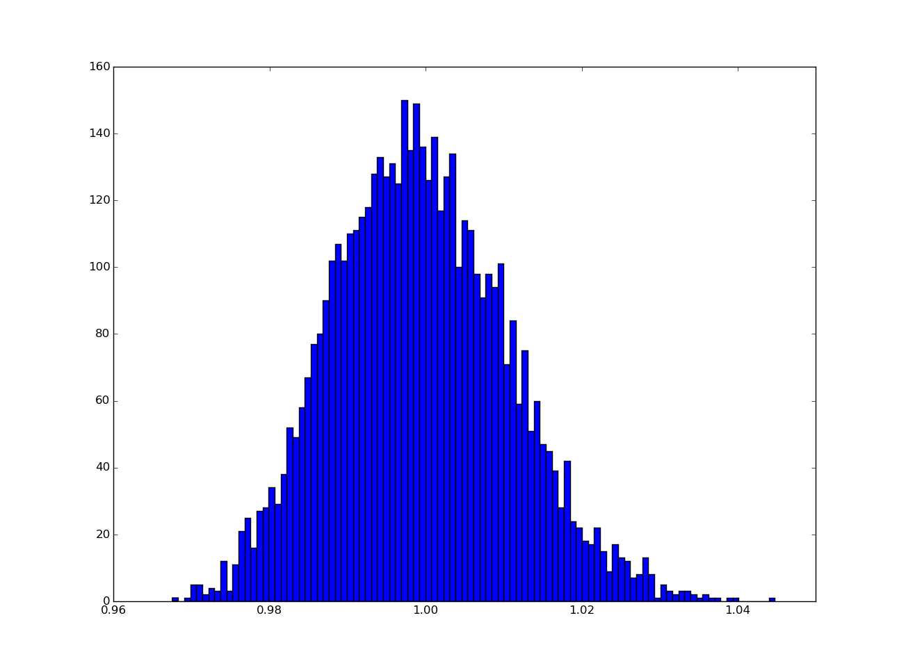
To reduce OCaPi calculation times from seconds to milliseconds, we generated 1 million random pick lists and used OCaPi to give each list a “label”: the calculated travel time. Then we fed the coordinates of the pick lists along with the travel times into a convolutional neural network. To train the networks we used the popular Caffe neural network framework linked with NVIDIA’s cuDNN convolutional neural network library running on two NVIDIA Tesla K80 GPU Accelerators (total four GPUs). By training four models in parallel (one on each GPU) we were able to find a neural network architecture that was very accurate with just a few weeks of effort. The network estimation of travel times is off by an average of 32.25 seconds for every hour of calculated travel time, a negligible amount when one considers all the factors that influence actual pick performance. See Figure 6 for more notes on accuracy.
Training and Computing Time Improvement
The whole point of this exercise was to make the OCaPi travel time estimation faster. So how did we do? We ran these experiments on a machine with two Intel Xeon E5-2640 and two NVIDIA Tesla K80 accelerators. We linked Caffe against cuDNN v2 and OpenBLAS compiled from source.
The first compute time hurdle was the training. With the Tesla K80 accelerators, we were able to update the network with one million training examples in just 52.6 seconds compute time, a speedup of a factor of 20 compared to the CPU (see Table 1).
| Intel Xeon E5-2640 with OpenBLAS | NVIDIA k80 linked against cuDNN v2 |
|---|---|
| 1090.741s | 52.556s |
For the travel time estimate, which is just a forward pass through the network (also known as a neural network inference; see the recent post Inference: The Next Step in GPU-Accelerated Deep Learning) we found that since the network is fairly small we don’t get a significant speedup by using the GPU. This test should be taken with a grain of salt, since we didn’t link against [Intel’s MKL or cuDNN v3, the latest CPU and GPU libraries.
| # pick lists | OCaPi | CPU network | GPU network |
|---|---|---|---|
| 1 | 5.369 | 2.202e-3 | 1.656e-3 |
| 10 | 1.326 | 1.991e-4 | 1.832e-4 |
| 100 | 0.365 | 6.548e-5 | 5.919e-5 |
| 1000 | 3.086e-5 | 2.961e-5 | |
| 10000 | 2.554e-5 | 2.336e-5 |
Bringing It All Together
There are many places in the warehouse management process where this fast and accurate OCaPi travel time estimator can be applied, and I use the estimator to demonstrate how to solve the batching problem in the example from above. I wrote a very simple optimization algorithm based on simulated annealing which starts with 40 orders of 2 items each split randomly between two pick lists. For 40 orders, there are 
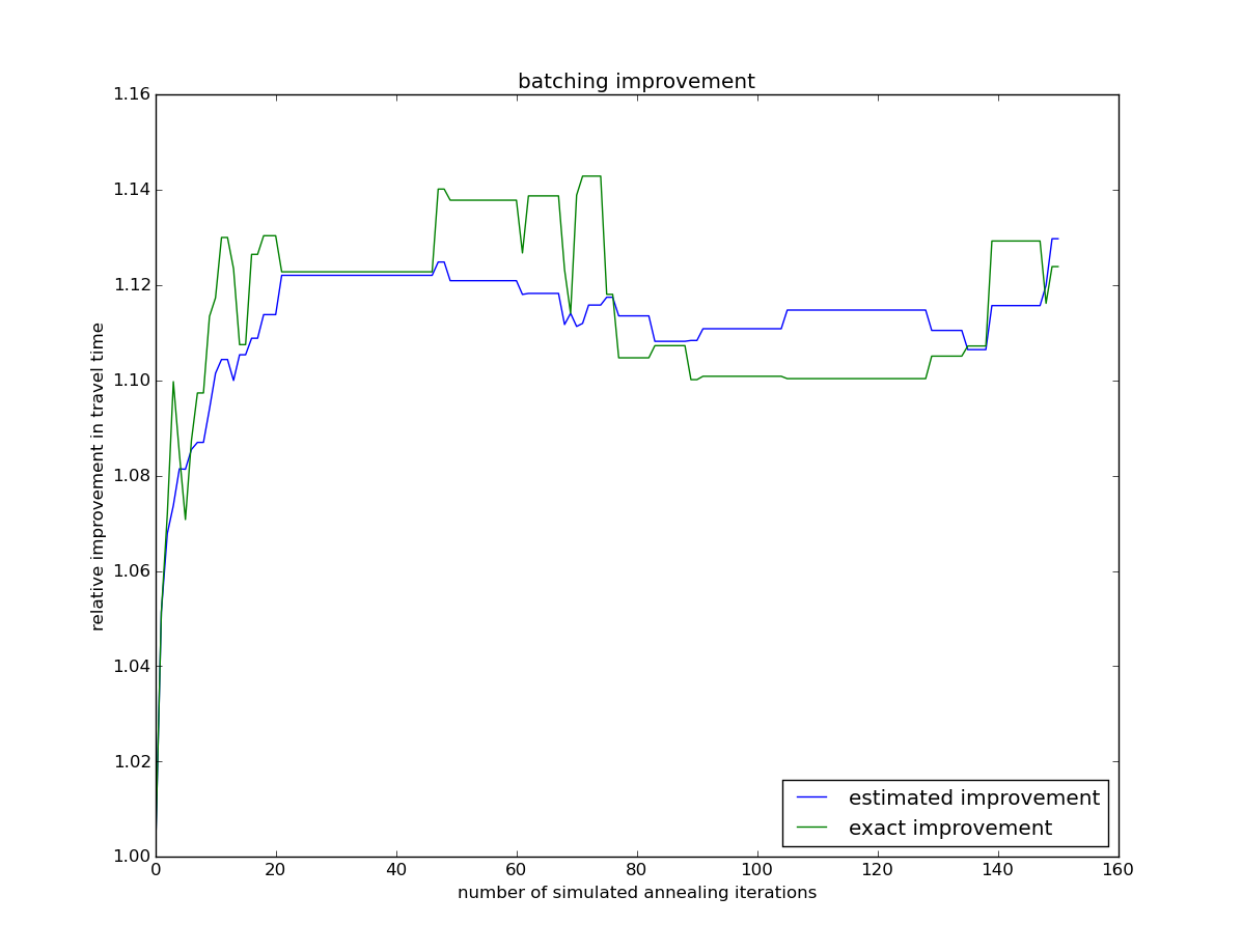
For the setting above and a realistic zone layout, optimized batches allowed the workers to decrease their travel time per item picked by an average of 11%, compared with a random batch. Clearly the actual benefit in production depends highly on the order pool, the number of zones, and other factors. What we see here is not a real-life improvement, but a very informative academic exercise.
Application to Any Black Box Algorithm
At first glance, this post would suggest that the key takeaway is our travel time estimation speedup and the better batches that can then be created. However, the same approach is applicable to many fields of industry and research: we were able to take an algorithm and, by treating it as a black box problem, transform it into a neural network that is very fast and ready to be deployed at scale on both CPU and GPU architectures. I am confident there are many other problems where this method can be applied, and I look forward to reading about exciting new breakthroughs powered by Neural Networks and GPUs.
Learn more about the exciting work being done at Zalando on our tech blog.
References
[1] Kees Jan Roodbergen, René de Koster, Routing order pickers in a warehouse with a middle aisle, European Journal of Operational Research, Volume 133, Issue 1, 16 August 2001, Pages 32-43, ISSN 0377-2217
[2] H. Donald Ratliff and Arnon S. Rosenthal, Order-Picking in a Rectangular Warehouse: A Solvable Case of the Traveling Salesman Problem, Operations Research, Vol. 31, No. 3 (May – Jun. 1983), pp. 507-521
[3] Kees Jan Roodbergen and René de Koster, Routing methods for warehouses with multiple cross aisles, International Journal of Production Research 39(9), 2001, pp. 1865-1883.
[4] Sebastian Henn, Sören Koch, and Gerhard Wäscher, Order Batching in Order Picking Warehouses: A Survey of Solution Approaches, January 2011, ISSN 1615-4274