[Note: Lung Sheng Chien from NVIDIA also contributed to this post.]
A key bottleneck for most science and engineering simulations is the solution of sparse linear systems of equations, which can account for up to 95% of total simulation time. There are two types of solvers for these systems: iterative and direct solvers. Iterative solvers are favored for the largest systems these days (see my earlier posts about AmgX), while direct solvers are useful for smaller systems because of their accuracy and robustness.
CUDA 7 expands the capabilities of GPU-accelerated numerical computing with cuSOLVER, a powerful new suite of direct linear system solvers. These solvers provide highly accurate and robust solutions for smaller systems, and cuSOLVER offers a way of combining many small systems into a ‘batch’ and solving all of them in parallel, which is critical for the most complex simulations today. Combustion models, bio-chemical models and advanced high-order finite-element models all benefit directly from this new capability. Computer vision and object detection applications need to solve many least-squares problems, so they will also benefit from cuSOLVER.
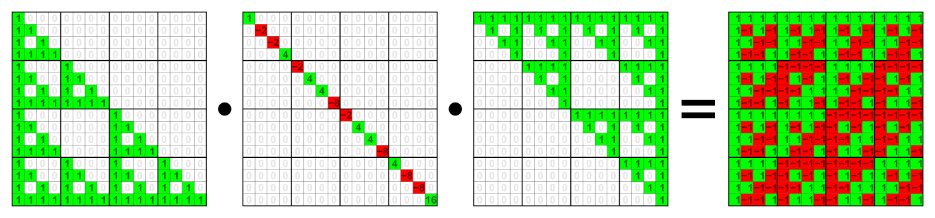
Direct solvers rely on algebraic factorization of a matrix, which breaks a hard-to-solve matrix into two or more easy-to-solve factors, and a solver routine which uses the factors and a right hand side vector and solves them one at a time to give a highly accurate solution. Figure 1 shows an example of 
In this post I give an overview of cuSOLVER followed by an example of using batch QR factorization for solving many sparse systems in parallel. In a followup post I will cover other aspects of cuSOLVER, including dense system solvers and the cuSOLVER refactorization API.
Overview of the cuSOLVER Library
The cuSOLVER library provides factorizations and solver routines for dense and sparse matrix formats, as well as a special re-factorization capability optimized for solving many sparse systems with the same, known, sparsity pattern and fill-in, but changing coefficients. A goal for cuSOLVER is to provide some of the key features of LAPACK on the GPU, as users commonly request LAPACK capabilities in CUDA libraries. cuSOLVER has three major components: cuSolverDN, cuSolverSP and cuSolverRF, for Dense, Sparse and Refactorization, respectively.
Let’s start with cuSolverDN, the dense factorization library. These are the most like LAPACK, in fact cuSOLVER implements the LAPACK API with only minor changes. cuSOLVER includes Cholesky factorization (potrf), LU factorization (getrf), QR factorization (geqrf) and Bunch-Kaufmann 
symtrf), as well as a GPU-accelerated triangular solve (getrs, potrs). For solving systems with QR factorization, cuSOLVER provides ormqr to compute the orthogonal columns of Q given A and R, and getrs to solve R. I’ll go into detail on these in a followup post.
cuSolverSP provides sparse factorization and solve routines based on QR factorization. QR can be used for solving linear systems and least-squares problems. QR factorization is very robust, and unlike LU factorization, it doesn’t rely on pivoting.
The cuSolverRF library can quickly update an existing LU factorization as the coefficients of the matrix change. This has application in chemical kinetics, combustion modeling and non-linear finite element methods. I’ll cover this more in a followup post.
For this post, I’ll take a deep look into sparse direct factorization, using the QR and batched QR features of cuSolverSP.
Key Performance Factors
Solving a sparse linear system is not just an arithmetic problem. To achieve the best performance on a given architecture, a sparse direct solver needs to consider multiple factors, and take steps to minimize the difficulties each presents.
- Minimize fill-in during factorization. To take advantage of the sparse nature of the original matrix A, we have to avoid ‘fill-in’ of the matrix with new non-zeroes during the factorization. The more fill-in, the lower the performance, since we are making more work with every new non-zero added. Furthermore, the fill-in can be so severe that a relatively small problem can consume all device memory, halting the factorization before we can get an answer. Reordering the matrix to reduce this fill-in can dramatically improve performance and increase the size of systems that we can solve using fixed resources.
- Discover and Exploit Parallelism. The symbolic analysis stage of a direct solver can build an ‘elimination tree’ of the matrix which shows independent paths of parallelism. The nodes of the tree with the same depth or ‘level’ can be computed simultaneously. Reordering the matrix may change the elimination tree, which changes the level of parallelism. Hence parallelism depends on the matrix structure if a reordering is given, and if a matrix cannot be reordered to extract parallelism, then maximum performance cannot be attained on modern many-core processors.
- Memory efficiency. Memory access patterns during numerical factorization are irregular, resulting in incoherent memory accesses which cannot achieve the potentially high bandwidth of a GPU. This is a key performance limiter in direct solvers.
- Index computation. Typically, indirect addresses are used to compute matrix factorizations, and addition operations are needed to compute the addresses of individual entries in the matrix storage format (dense or sparse). The data needed to compute these indices typically comes from global memory, which increases access latency.
Applying Graph Theory to Matrix Reordering
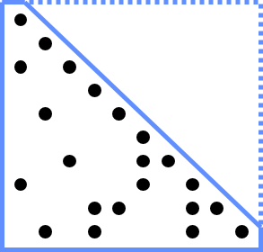
Graph theory plays an important role in calculations to reorder matrices in direct solvers. We would like to minimize fill-in and predict the final sparsity pattern of the numerical factorization. Both of these goals can be addressed using a ‘symbolic’ factorization—an analysis stage before the actual arithmetic is performed—plus a graph heuristic re-ordering of the columns of the matrix to minimize fill-in. The graph of a symmetric matrix like the matrix A in Figure 2 is undirected, meaning that for every connection of row i to column j there is a symmetric connection from row j to column i.

This means that every connection is a two-way street, and as shown in Figure 3, we don’t add arrows to connections in the graph, lines are enough. We can also store only half of the matrix, as the sparsity diagram in Figure 2 shows. This has many advantages, not least of which is we generally have only half as much work to do to factor a symmetric matrix because the factors are symmetric. You may have noticed that the
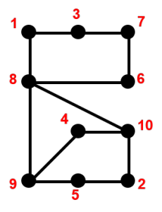
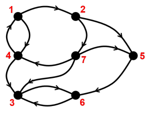
For non-symmetric matrices like the one in Figure 4, the graph is a directed graph, meaning each connection is a one-way street. For a directed graph we have to draw arrows for each connection to indicate which way it flows. This is the general case, and as you can see by the sparsity diagram on the left, we have to store potentially more information, and can’t take advantage of entries being repeated symmetrically. In this case we have to do the full amount of work, no short cuts.
Graph algorithms like Depth First Search (DFS) can be directly applied to the graph incarnation of the matrix. Finding a good fill-reducing ordering for a given matrix involves several calls to DFS. Two common algorithms in this class are Reverse Cuthill-McKee (RCM) for symmetric systems and Approximate Minimum Degree (AMD) for non-symmetric systems. An upcoming update to cuSOLVER will provide these ordering routines. By reducing the fill-in, we arrive at the same solution faster and using much less memory.
Maximizing Parallelism by Minimizing Pivoting
You might remember my earlier comment about “when the factors exist”. To see what can go wrong, let’s make an analogy to high-school algebra. We want to factor an equation 


In linear algebra, we have the same possibility, the matrix could just be ‘unsolvable’, meaning it doesn’t contain the information we need to find x uniquely. We would see this during factorization as a breakdown of the algorithm where it would need to divide by zero, or by a number so numerically close to zero that the computer treats it as zero. To avoid this we can try several approaches, the most direct of which is called ‘pivoting’, or re-ordering the columns of the matrix so a non-zero value is used in the division instead of the zero value. We still get the same answer in the end, but we have to do some book-keeping to remember what columns have been swapped.
In certain circumstances, performance is limited by pivoting. For example, the pivoting strategy in LU factorization requires searching each row that needs to pivot for a ‘valid’ column. The row searches are sequentially dependent: each row search must wait for all previous rows to be finished (columns to be swapped), which limits parallelization. We wish to avoid the need for pivoting, or reduce it as much as possible by reordering the matrix to move large-magnitude elements to the diagonal. This is known as ‘static pivoting’, and it can greatly increase parallelism in LU factorization. We can’t prove that this always works, but a combination of static pivoting and adding a small value on the diagonal when a numerically small pivot is encountered seems to be as robust as pivoting in tests. The price we pay to avoid work during the factorization is that we must do extra work in the solve phase to be sure the solution is accurate enough.
Improving Memory Coherence
Once a matrix with a certain reordering is given, we can improve memory efficiency by clever factorization algorithms. Traditional “supernodal” or “multifrontal” algorithms can gather sparse data to form blocks and apply efficient BLAS2/BLAS3 operations. This improves memory efficiency on BLAS operations but does not improve the memory efficiency for gathering. If a supernode or front is big enough, the time spent in computation is much bigger than the time required for data transfer, and by overlapping the communication with computation the supernodal or multifrontal algorithm is a win.
In the case that the matrix does not have big supernodes or fronts, we need another way to improve performance.
If only one linear solve is needed, for a single right hand side or a single matrix, there is not much we can do. But if we have a large enough set of linear systems to solve, the situation is different.
A Batched Linear Solver Approach
Let’s consider a set of 


- Only one symbolic factorization stage is needed to predict the sparsity structure of the numerical factors independent of the numerical values in each matrix.
- Index computation overhead goes down because all batched operations share the same index to query the data.
- Each linear system can be solved independently, so parallelism comes from both the sparsity pattern of the matrix and trivially parallel batched operations.
- Memory efficiency can be improved by reorganizing the data layout in memory.
cuSOLVER provides batch QR routines to solve sets of sparse linear systems. cuSOLVER’s QR factorization is a simple ‘left-looking’ algorithm, not a supernodal or multifrontal method. However with high memory efficiency and extra parallelism from batch operations, batch QR can reach peak bandwidth if 
How to use Batch QR in cuSolverSP
Let’s walk through a use case for batch QR.
Step 1: prepare the matrices, right-hand-side vectors and solution vectors. cuSolverSP require an ‘aggregation’ layout which concatenates the data one after another. For example, 


Step 2: create an opaque info structure using cusolverSpCreateCsrqrInfo()
Step 3: perform analysis using cusolverSpXcsrqrAnalysisBatched(), which extracts parallelism and predicts the sparsity of the to-be-created 

Step 4: Find the size of buffer needed by calling cusolverSpDcsrqrBufferInfoBatched(). There are two different buffers, one is an internal data buffer and the other is working space needed for the factorization. The internal buffer is created and kept in the opaque info structure. The size depends on the sparsity of the matrix and the chosen batch size. You should verify that the available device memory is sufficient for the internal buffer. If it is not, you may need to reduce the batch size until the size of the internal buffer is less than the available device memory. On the other hand, the working space is volatile, so you can reuse it for other computations.
Step 5: allocate working space explicitly using cudaMalloc(). The internal buffer is allocated automatically.
Step 6: Solve the set of linear systems by calling cusolverSpDcsrqrsvBatched(), which computes 
Performance of Batch QR
We tested the performance of batched QR factorization on 25 matrices from the Florida Sparse Matrix Collection (http://www.cise.ufl.edu/research/sparse/matrices/ ). The matrices cover a range of sizes and sparsity patterns: some small matrices that can fit into L2 cache; some matrices with large zero fill-in; some matrices with very little parallelism.
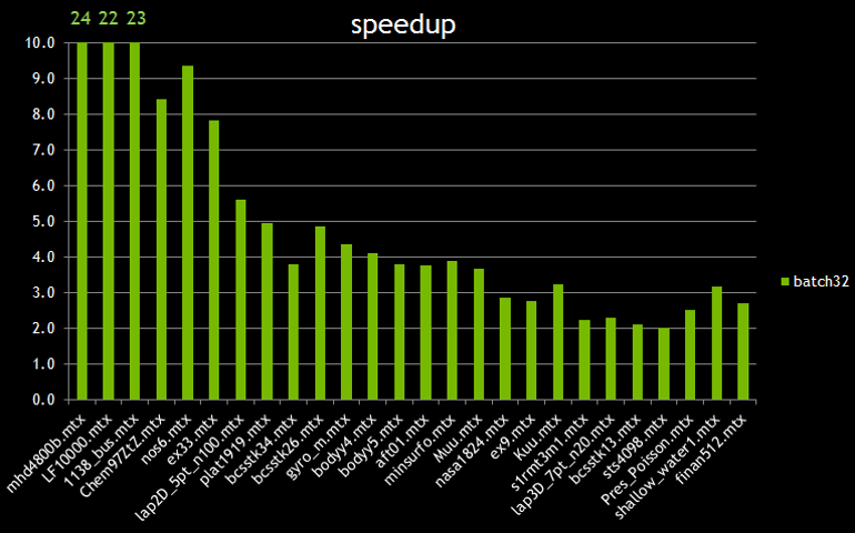
Figure 5 compares the performance of a single QR factorization with the performance of batch QR with a batch size of 32. The speedup is the ratio between 32*Time(QR) and Time(batch QR). The x-axis is roughly in order of the density of fill-in. We see good speedup up to 24x when the density of fill-in is small; As the density of fill-in goes up, the performance of batchQR goes down because of more pressure on memory I/O, reducing the ratio of computation to communication.
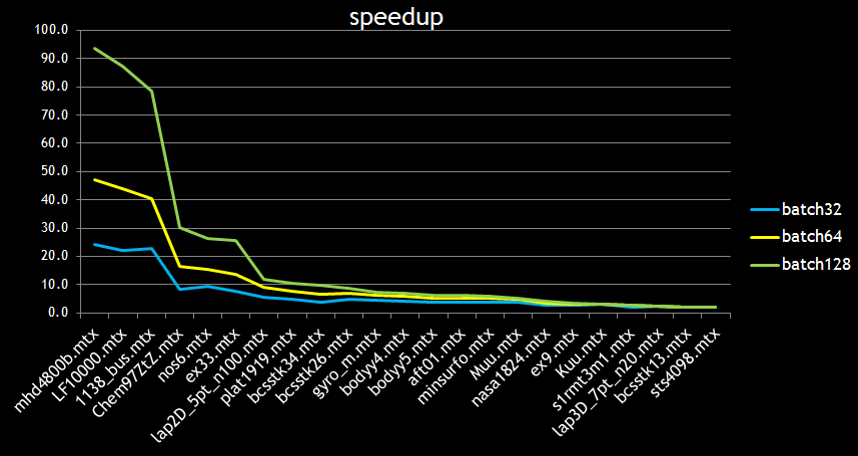
Figure 2 shows the performance of batch QR for three different batch sizes: 32, 64 and 128. It is clear that batch QR has excellent performance when the fill-in is small. In this regime, the runtime is the same independent of the batch size until we reach the peak bandwidth possible on the device; this is a consequence of “the bigger the batch, the more parallelism available”.
Conclusion
Direct solvers are a new powerful feature in CUDA 7.0. Modern GPU devices have huge bandwidth and floating point throughput, but sparse direct solvers are a challenge because of insufficient parallelism, random access patterns and fill-in of the sparsity pattern. We demonstrated the batch QR factorization approach can naturally increase parallelism and improve memory access efficiency, especially when fill-in is not severe. Batch QR can also be used to solve eigenvalue problems, and to solve many least-squares problems in parallel. Please tell us about your uses for cuSOLVER in the comments!
Want to learn more?
To get started with cuSOLVER, first download and install the CUDA Toolkit version 7.0. There are more detailed batch QR examples available in the online CUDA documentation. You should also check out the session “Jacobi-Davidson Eigensolver in cuSOLVER Library” from GTC 2015. Try cuSOLVER today!