NVIDIA’s Turing GPUs introduced a new hardware functionality for computing optical flow between images with very high performance. The Optical Flow SDK 1.0 enables developers to tap into the new optical flow functionality. You can download the Optical Flow SDK 1.0 from the NVIDIA developer zone.
Until a few years ago, tasks such as recognizing and tracking an object or classifying an action in video streams were out of reach for computers due to the complexity involved. With the advent of DNNs and massive acceleration made possible by GPUs, all these tasks can now be performed by computers with high accuracy.
Two primary methods exist to track objects within a video feed.
- Detect in every frame: Identify the bounding box for the object(s) of interest in each frame using object classification and track the object boundaries from frame to frame.
- Detect and track: Identify the bounding box for the object in the first frame (or every nth frame) and calculate the motion of the pixels (or blocks) belonging to the object in the subsequent frames for tracking
The first method is accurate but computationally complex since object classification (inference) needs to be run on each frame. The second method requires less computation but relies on accurate estimate of the motion/flow vectors of pixels (or blocks) between successive frames.
The two types of optical flow typically used in object tracking include dense optical flow and sparse optical flow. The latter is popular because of its low computational complexity and usefulness in methods such as Kanade-Lucas-Tomashi (KLT) feature trackers. Dense optical flow methods provide higher accuracy with greater computational complexity. Due to this, dense optical flow computation has been out of reach for many practical use-cases. Other use-cases for optical flow include stereo depth estimation, video frame interpolation and video frame extrapolation.
The hardware optical flow functionality in Turing GPUs helps all these use-cases by offloading the intensive flow-vector computation to a dedicated hardware engine on the GPU silicon. This frees up GPU and CPU cycles for other tasks. NVIDIA’s Optical Flow SDK exposes a new set of APIs which give developers access to this hardware functionality.
Evolution of Optical Flow
NVIDIA GPUs from Maxwell, Pascal, and Volta generations include one or more video encoder (NVENC) engines which provided a mode called Motion-Estimation-only mode. This mode allowed users to run only motion estimation on NVENC and retrieve the resulting motion vectors (MVs). The motion estimation hardware searches the neighboring areas, and picks the closest matching block. The criteria for closest match is tuned for optimizing the encoding cost, i.e. bits consumed by the residual after motion compensation. Due to this method, motion vectors may not be very accurate in many use-cases which require tracking precision. This is particularly true in varying lighting conditions in which intensity changes from one frame to the next.
The optical flow hardware in Turing GPUs uses sophisticated algorithms to yield highly accurate flow vectors. These algorithms effectively handle frame-to-frame intensity variations and also track the true object motion much more closely than the traditional ME-only mode of NVENC. Table 1 shows the differences between Turing’s optical flow and the traditional ME-only mode of NVENC.
Table 1. Differences between Turing Optical Flow and Traditional ME-only mode of NVENC
| Turing Optical Flow | Maxwell/Pascal/Volta NVENC Motion Vectors | |
| Granularity | Up to 4×4 | Up to 8×8 |
| Accuracy | Close to true motion Low average EPE (end-point error) |
Optimized for video encoding; may differ from true motion Higher EPE |
| Intensity changes | Robust to intensity changes | Not robust to intensity changes |
| Software | Optical Flow SDK 1.0+, Q1 2019 | Video Codec SDK 7.0+, Available |
Optical Flow SDK
Functionality
The optical flow hardware in the Turing GPUs returns flow vectors at a granularity as high as 4×4 pixel blocks with quarter-pixel accuracy. The accuracy and granularity can be further improved using various post-processing algorithms. The Optical Flow SDK includes optimized implementations for some of the popular post-processing algorithms. These algorithms run by default as part of slow preset using CUDA cores in the Optical Flow SDK 1.0.
The software libraries required to access the optical flow hardware will be included in the NVIDIA display driver. The SDK incorporates the C-API definition, documentation, and sample applications with reusable classes. The API is uniform across Windows and Linux operating systems when accessed via CUDA interfaces. The library also exposes a dedicated DirectX 11 API for Windows-specific use-cases, supported on Windows 8.1 and Windows 10.
The Optical Flow API consists of three major functions: Init, Execute and Destroy, as shown below.
NV_OF_STATUS(NVOFAPI* PFNNVOFINIT) (NvOFHandle hOf,
                                    const NV_OF_INIT_PARAMS *initParams);

NV_OF_STATUS(NVOFAPI* PFNNVOFEXECUTE) (NvOFHandle hOf,
                                       const NV_OF_EXECUTE_INPUT_PARAMS *executeInParams,
                                       NV_OF_EXECUTE_OUTPUT_PARAMS *executeOutParams);

NV_OF_STATUS(NVOFAPI* PFNNVOFDESTROY) (NvOFHandle hOf);
Besides the three basic functions, there are functions for CUDA and D3D11 buffer management.
The classes NvOF, NvOFCuda and NvOFD3D11 included in the SDK provide classes which can be directly used by the applications or derived from. As an example, a typical application with CUDA buffers may be written as shown below.
// Initialize a data loader for loading frames
std::unique_ptr dataLoader = CreateDataloader(inputFileName);

// Create Optical Flow object with desired frame width and height
NvOFObj nvOpticalFlow = NvOFCuda::Create(cuContext,
   Width,
   Height,
   NV_OF_BUFFER_FORMAT_GRAYSCALE8,
                                            NV_OF_CUDA_BUFFER_TYPE_CUARRAY,
                                            NV_OF_CUDA_BUFFER_TYPE_CUARRAY,
                                            NV_OF_MODE_OPTICALFLOW,
                                            NV_OF_PERF_LEVEL_SLOW,
                                            inputStream,
                                            outputStream);

// Create input and output buffers
inputBuffers = nvOpticalFlow->CreateBuffers(NV_OF_BUFFER_USAGE_INPUT, 2);
outputBuffers = nvOpticalFlow->CreateBuffers(NV_OF_BUFFER_USAGE_OUTPUT, 1);

.
.
.

// Read frames and calculate optical flow vectors on consecutive frames
for (; !dataLoader->IsDone(); dataLoader->Next())
{
    inputBuffers[curFrameIdx]->UploadData(dataLoader->CurrentItem());

    nvOpticalFlow->Execute(inputBuffers[curFrameIdx ^ 1].get(),
                                        inputBuffers[curFrameIdx].get(),
                                        outputBuffers[0].get());

    outputBuffers[0]->DownloadData(pOut.get());

    // Use the flow vectors generated in buffer pOut.get() for further
    // processing or save to a file.

    curFrameIdx = curFrameIdx ^ 1;
}
For more details, please refer to the Samples folder in the SDK.
In addition to the C-API, NVIDIA will support the hardware accelerated optical flow functionality in various deep learning frameworks such as Pytorch and Caffe for ease of access by deep-learning applications.
Using Optical Flow on Decoded Frames from NVDEC
Training deep learning networks for video post-processing with optical flow information represents a common use case. The video frames decoded by GPU’s NVDEC (on-chip video decoder) engine can be passed to the optical flow engine for generating optical flow vector maps between desired pairs of frames as part of training. These maps provide auxiliary information to the video post-processing network.
Passing the video frames decoded by NVDEC to the optical flow engine currently requires copyingvideo frames decoded using NVDECODE API into video memory for processing by the optical flow hardware. This can be accomplished as follows:
// Create Optical Flow object with desired frame width and height
NvOFObj nvOpticalFlow = NvOFCuda::Create(cuContext,
   Width,
   height,
                                        NV_OF_BUFFER_FORMAT_GRAYSCALE8,
                                            NV_OF_CUDA_BUFFER_TYPE_CUARRAY,
                                            NV_OF_CUDA_BUFFER_TYPE_CUARRAY,
                                        NV_OF_MODE_OPTICALFLOW,
                                        NV_OF_PERF_LEVEL_FAST,
                                            inputStream,
                                            outputStream);

// Create input and output buffers
inputBuffers = nvOpticalFlow->CreateBuffers(NV_OF_BUFFER_USAGE_INPUT, 2);
outputBuffers = nvOpticalFlow->CreateBuffers(NV_OF_BUFFER_USAGE_OUTPUT, 1);

// Convert NV12 decoded frames to grayscale image for optical flow.
// NV12 -> grayscale conversion is just copy of luma plane.
CUDA_DRVAPI_CALL(cuCtxPushCurrent(cuContext));
CUDA_MEMCPY2D cuCopy2d;
memset(&cuCopy2d, 0, sizeof(cuCopy2d));
cuCopy2d.srcMemoryType = CU_MEMORYTYPE_DEVICE;

// Copy the decoded frame returned from cuvidMapVideoFrame
// to CUArray which will be used by Optical Flow engine.
//
// CUDA device pointer returned by cuvidMapVideoFrame(...)
cuCopy2d.srcDevice = pDecodeFrameDevPtr;
// Decoded frame pitch returned by cuvidMapVideoFrame(...)
cuCopy2d.srcPitch = decodeFramePitch;

cuCopy2d.dstMemoryType = CU_MEMORYTYPE_ARRAY;
cuCopy2d.dstArray = inputBuffers[curFrameIdx]->getCudaArray();
cuCopy2d.WidthInBytes = width;
cuCopy2d.Height = height;

// Kick-off async copy
CUDA_DRVAPI_CALL(cuMemcpy2DAsync(&cuCopy2d, inputStream));
CUDA_DRVAPI_CALL(cuCtxPopCurrent(&cuContext));

// Run Optical Flow
nvOpticalFlow->Execute(inputBuffers[curFrameIdx ^ 1].get(),
        inputBuffers[curFrameIdx].get(),
        outputBuffers[0].get());
Accuracy of Flow Vectors
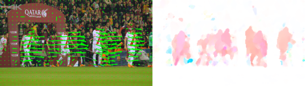
An objective measure of the accuracy of the flow vectors returned by the hardware can be obtained by comparing the vectors with ground truth, if available. We used the KITTI Vision Benchmark Suite 2012 and 2015, MPI Sintel, and Middlebury Computer Vision datasets which make available ground truth flow vectors.
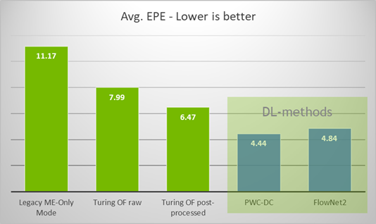
We measured the average end-point error (EPE) using the KITTI Flow 2015 . The EPE for a flow vector is defined as the Euclidean distance between the hardware-generated flow vector and the ground-truth flow vector. Figure 1 shows the average EPE of various algorithms. The average EPE obtained using a couple of popular DL-based optical flow methods is also shown for comparison. The average EPE from Turing’s optical flow hardware is comparable to some of the best-known DL methods with performance increases of 7x-10x without utilizing any CPU or CUDA cores.
Although the Optical Flow hardware uses sophisticated algorithms for computing the flow vectors, situations exist in which the generated flow vectors may not be reliable. For example, if the input frame reveals an object occluded in the reference frame, the optical flow vectors for some of the surrounding pixels/blocks may be inaccurate. The Optical Flow API returns a buffer consisting of confidence levels (called cost) for each of the flow vectors to deal with these situations. The application can use this cost buffer to selectively accept or discard regions of the flow vector map.
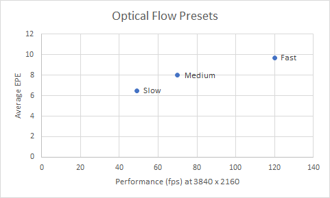
Accuracy vs Performance
The optical flow API exposes three presets which allow users to trade performance for accuracy. Figure 2 shows the operating points for the presets.
End-to-end Evaluation
Now let’s look at the results of two end-to-end use-cases developed to evaluate the usefulness of the optical flow functionality.
Video Action Recognition
In this evaluation, we modified a video action recognition (aka “video comprehension”) DNN to use the optical flow vectors returned by the Turing GPU hardware as auxiliary information. Figure 3 compares the inference error rate obtained on the UCF101 video dataset with and without optical flow versus performance in each case.
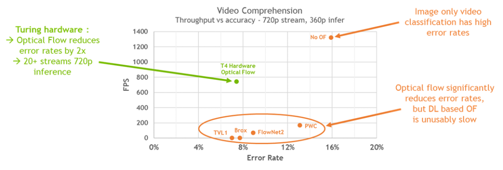
The video action recognition error rate of the Turing-optical-flow assisted network shown in the above chart is significantly lower than the error rate without optical flow and comparable with some of the best methods. The Turing hardware achieves this at very high performance (~750 fps at 720p decode + 360p infer).
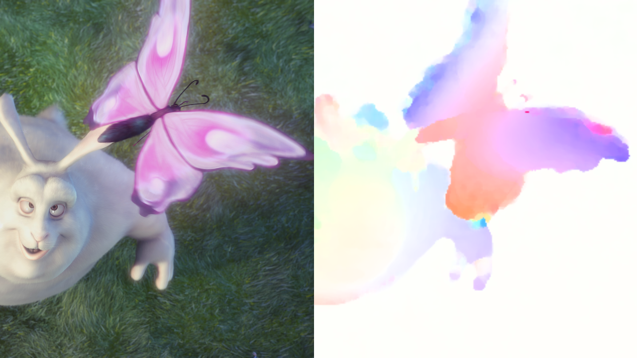
Video Frame Rate Upconversion
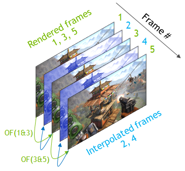
Figure 4 shows the basic concept of video frame rate upconversion. The hardware generates every alternate frame using optical flow vectors to double the effective frame rate of the video. This technique improves smoothness of video playback or increases the game/graphics rendering speed on low-end hardware.
Let’s examine how this works. First, the Turing hardware computes the optical flow vectors between frames 1 and 3 (two successive rendered frames). Next, the flow vectors are validated for accuracy and reliability using cost returned by the API. This step ensures that low-confidence outliers are discarded. The remaining high-confidence flow vectors are then used to warp frame 1 at half the temporal distance between frames 1 and 3. Finally, macroblock interpolation is used to fill in the missing parts of the image to construct completed frame 2. The same procedure can be applied in reverse temporal order (calculating flow vectors from frame 3 to frame 1 and then constructing the middle frame) in order to improve the interpolation further. Additional post-processing can be used to construct the final video frame 2.
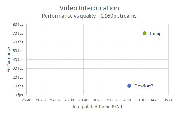
We implemented this method and evaluated the quality of the resulting interpolated frames using objective measures such as PSNR and SSIM. Figure 5 shows that the Turing-optical-flow-assisted frame-rate upconversion provides 7x higher performance than Flownet2-assisted frame-rate upconversion with ~1 dB higher PSNR. This makes it possible to run video frame rate upconversion algorithm in real-time, something previously impossible.
Obtaining the Optical Flow SDK
The Optical Flow SDK 1.0 can now be downloaded from the developer page. For any questions, please contact video-devtech-support@nvidia.com.