This blog dives into a theoretical machine learning concept called the bias variance decomposition. This decomposition is a method which examines the expected generalization error for a given learning algorithm and a given data source. This helps us understand questions like:

How can I achieve higher accuracy with my model without overfitting?
Why are my results so unstable? If I change the test set my performance changes dramatically!

Generalization concerns overfitting, or the ability of a model learned on training data to provide effective predictions on new unseen examples. We perform experiments using two popular tree ensemble learning algorithms, Gradient Boosting and Random Forests, and examine how a range of hyperparameters for these models affects the decomposition of expected prediction error for a regression problem.

We assume you have some prior knowledge of Gradient Boosting or Random Forests. You will learn conceptually what are bias and variance with respect to a learning algorithm, how gradient boosting and random forests differ in their approach to reducing bias and variance, and how you can tune various hyperparameters to improve the quality of your model.

These experiments all use the XGBoost library as a back-end for building both gradient boosting and random forest models. Code for all experiments can be found in my Github repo. See my previous post on XGBoost for a more detailed explanation for how the algorithm works and how to use GPU accelerated training.

Bias Variance Decomposition Explained

The expected prediction error in this article refers to the expected value of mean squared error:

$Err(x)=E[(y-\hat{f}(x))^2]%0$

Here $\hat{f}(x)%0$ is the model learned, $y%0$ represents the target label, and $x%0$ represents an unseen test example. $\hat{f}(x)%0$ is a random variable and represents the model trained on some randomly drawn samples from a data source. The model is typically trained on some fixed number of examples in each trial in our experiments.

It is important to understand that this equation does not describe the error of a single model such as you might get from evaluating a single test/train split. It instead describes the average error if we hypothetically built many different models by sampling a data source and then evaluating on an independent test set.

We will also make the assumption that the label $y%0$ is generated as follows:

$y=f(x)+\varepsilon%0$

Where $f(x)%0$ represents the true function that we are trying to learn. The labels will contain Gaussian noise with mean 0 and variance $\sigma^2%0$ . You can think of our task as learning $f(x)%0$ as closely as possible given some training data with n training instances exhibiting target values provided by f(x) that have been corrupted by noise.

The expected prediction error is decomposed into the following terms:

$Err(x)=Bias(\hat{f}(x))^2+Var(\hat{f}(x))+\sigma^2%0$

Where:

$Bias(\hat{f}(x))=E[\hat{f}(x)]-f(x)%0$

$Var(\hat{f}(x))=E[\hat{f}(x)^2]-E[\hat{f}(x)]^2%0$

We will not perform the actual derivation of how we got these components; if you’re interested you can read this derivation. The most important thing is to understand conceptually what these different components represent.

Bias represents on average, across training sets, how far away our learned model predictions $\hat{f}(x)%0$ are from the true function $f(x)%0$ . Typically the bias of your model will be high if it does not have the capacity to represent what is going on in $f(x)%0$ . For example if $f(x)%0$ was a quadratic function and we used a linear model for $\hat{f}(x)%0$ the predictions may be quite far from the true function for many values of $x%0$ .

The variance represents how much your learned model changes if you train it on a different sample of data. Intuitively we can see that high variance is undesirable by considering that the true function $f(x)%0$ we are trying to approximate never changes. If your model changes dramatically when you train on different subsamples of data it can mean the learning algorithm is very sensitive to noise in the training data or is inherently unstable.

The third component $\sigma^2%0$ is called the irreducible error, and as the name implies, we will not be able to reduce this component by choice of learning algorithm. It arises as some source of noise such as measurement error.

So how can we experimentally evaluate this decomposition? We use a data generator for which we know exactly the true function $f(x)%0$ and noise component $\sigma^2%0$ . In general it is not possible to do this decomposition for real data for two reasons:

We do not know how to separate the true function and noise (if we knew the true function we probably would not be learning a model)
Real datasets typically have a finite number of examples. For these experiments we need to draw completely independent training examples from the data source for each model we build.

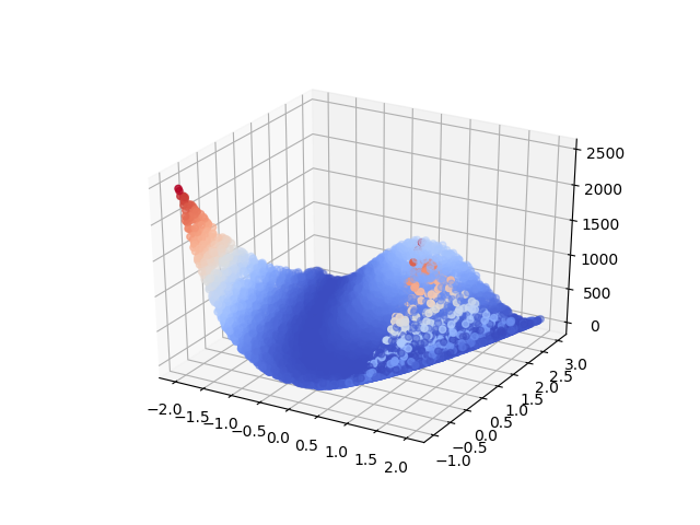
Our experiments use the two-dimensional Rosenbrock function as our data source, visualized in figure 1. The choice of function here is somewhat arbitrary; we use this function because it is easy to visualize and provides some challenge to the learning algorithm by variation in its surface.

rosenbrock function image — Figure 1. Rosenbrock test function

Experimental Methodology

Our experiments train each model on 1000 training examples (unless otherwise stated), drawn uniformly from the generator, generating 100 independent models. $\sigma%0$ is set to 100 in all cases. Predictions for unseen examples are performed on an independently drawn test set of size 10000. We report single values for the $Bias^2%0$ and $Variance%0$ representing the expected value of these terms over the entire test set.

The XGBoost library is used to generate both Gradient Boosting and Random Forest models.

Code for reproducing these experiments can be found here. We use XGBoost’s sklearn API to define our models. Each figure in this post is followed by the code used to specify models for that particular experiment.

Gradient Boosting

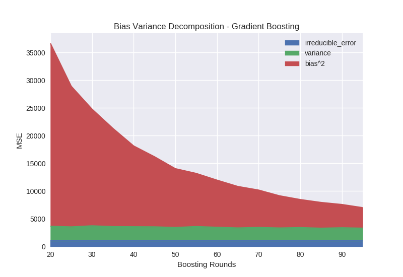
The first parameter we explore for gradient boosting is the number of boosting rounds, in which each round corresponds to the addition of a new decision tree. Recall that the goal of boosting is the progressive refinement of the model over time, with each new tree compensating for error in the previous model. Figure 2 shows the bias term consistently decreasing as we increase the number of rounds from 20 to 100 while the variance remains relatively unchanged.

Python code specifying models from figure 2:

n_estimators_range = range(20, 100, 5)
models = [xgb.XGBRegressor(n_estimators=n_estimators) for n_estimators in n_estimators_range]

The learning rate parameter (sometimes known as shrinkage) directly controls the strength of each new tree by scaling the output weights in each leaf. If the learning rate is set to a low value instead of a higher value, it requires an appropriately increased number of boosting rounds to achieve the model capacity. Figure 3 shows the effect of learning rates between 0.1 and 1.0 for a fixed number of boosting rounds (100).

The variance of the model decreases significantly as we decrease the learning rate. Intuitively, models fit using a high learning rate more aggressively capture variation between different training samples, leading to undesirable variance in the model. If the learning rate is set too low, the bias starts to rise because the model is not able to fit quickly enough in the given number of iterations.

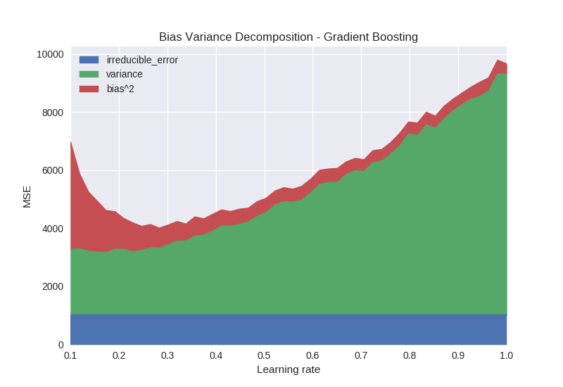
bias variance decomposition gradient boosting learning rate graph — Figure 3. Gradient Boosting – Learning Rate

Figure 3. Gradient Boosting – Learning Rate

Python code specifying models from figure 3:

learning_rate_range = np.linspace(0.1, 1.0)
models = [xgb.XGBRegressor(learning_rate=learning_rate) for learning_rate in
              learning_rate_range]

From these observations we see that gradient boosting has mechanisms for reducing both bias and variance in the expected prediction error. We can combine these to train a model with a low learning rate and a high number of rounds to obtain both low bias and variance. This hints at why gradient boosting can be such a powerful general-purpose learning algorithm.

Two hyperparameters often used to control for overfitting in XGBoost are lambda and subsampling.

The lambda parameter introduces an L2 penalty to leaf weights via the optimisation objective. This is very similar to ridge regression. The penalty helps to shrink extreme leaf weights and can stabilise the model at the cost of introducing bias. We often discuss bias variance decomposition in terms of a trade-off between the bias and variance terms. As we can see in Figure 4 this is true for the lambda parameter. Variance decreases as the penalty is increased at the cost of increased bias. One other interesting property of the lambda parameter is that it introduces numerical stability in software implementation. We can see that a very small value of lambda is beneficial over 0. The reason why this occurs is the leaf weights for the tree are calculated as $-\frac{G}{H+\lambda}%0$ (see here for details). When the denominator of this expression becomes close to 0, numerical instability occurs, so some small value of lambda can guard against this.

bias variance decomposition gradient boosting lambda l2 penalty graph — Figure 4. Gradient Boosting – Lambda (L2 penalty)

Python code specifying models from figure 4:

reg_lambda_range = np.linspace(0.001, 20.0)
models = [xgb.XGBRegressor(max_depth=15, reg_lambda=reg_lambda) for reg_lambda in
              reg_lambda_range]

The subsample parameter refers to stochastic gradient boosting, in which each boosting iteration builds a tree on a subsample of the training data. Figure 5 shows that bias is not greatly affected by the use of subsampling until the sample size gets close to 0.1 and the algorithm is no longer able to accurately fit the data. The primary effect of subsampling is on the variance of the output model, with a “sweet spot” for this dataset occurring somewhere between 0.3-0.6. An explanation for this phenomenon is that the algorithm can be prevented from over fitting to a particular training instance or group of training instances over multiple iterations by changing the available training sample at each iteration.

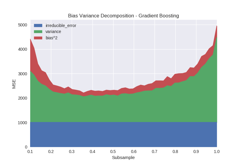
bias variance decomposition gradient boosting subsample graph — Figure 5. Gradient Boosting – Subsample

Python code specifying models from figure 5:

subsample_range = np.linspace(0.1, 1.0)
models = [xgb.XGBRegressor(max_depth=15, reg_lambda=0.01, subsample=subsample) for subsample in
              subsample_range]

Random Forests

Both random forests and gradient boosting produce ensembles of trees but the mechanisms by which they reduce expected prediction error differ.

Figure 6 shows the effect of the number of trees in a random forest model. Increasing the number of trees has the effect of reducing variance. This is because each tree in a random forest is built with variation introduced by sampling both training rows and features. The output prediction is an average over all models and tends to stabilise as the number of models being averaged increases.

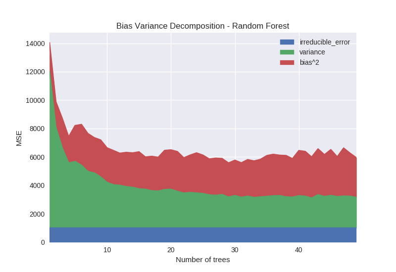
bias variance decomposition random forest number of trees graph — Figure 6. Random Forest – Number of trees

Python code specifying models from figure 6:

n_estimators_range = range(1, 50) models = [xgb.XGBRFRegressor(max_depth=12, n_estimators=n_estimators) for n_estimators in
              n_estimators_range]

Figure 7 shows the effect of the max depth parameter on random forest models. Bias is clearly and dramatically reduced as the depth of the tree is increased. This is because the capacity of the model is increasing exponentially with depth. At each additional level in the binary tree the possible number of leaves is doubled. As each leaf outputs a unique prediction, the capacity of the model to fit complex functions increases with depth.

As the random forest model cannot reduce bias by adding additional trees like gradient boosting, increasing the tree depth will be the primary mechanism of reducing bias. For this reason random forest models may need to be significantly deeper than their gradient boosted counterpart to achieve similar accuracy (in many cases boosted decision stumps can be extremely accurate).

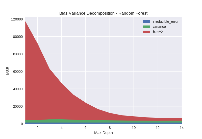
bias variance decomposition random forest max depth graph — Figure 7. Random Forest – Max Depth

Python code specifying models from Figure 7:

max_depth_range = range(1, 15) models = [xgb.XGBRFRegressor(max_depth=max_depth, reg_lambda=0.01) for max_depth in
              max_depth_range]

Given that we use the XGBoost back-end to build random forests, we can also observe the lambda hyperparameter. Figure 8 shows that increasing the lambda penalty for random forests only biases the model. This seems like a surprising result. The difference in performance between gradient boosting and random forests occurs because the gradient boosting process is able to take many steps towards the optimisation objective. Introducing a regularisation penalty to gradient boosting limits the size of each optimisation step but given sufficient iterations the algorithm will still converge towards some minimum. The random forest model gets only one optimisation step to generate the best model; constraining this step simply results in a suboptimal model.

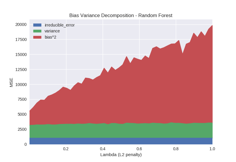
bias variance decomposition random forest lambda l2 penalty graph — Figure 8. Random Forest – Lamba (L2 penalty)

Python code specifying models from Figure 8:

reg_lambda_range = np.linspace(0.001, 1.0) models = [xgb.XGBRFRegressor(max_depth=15, reg_lambda=reg_lambda) for reg_lambda in reg_lambda_range]

Lastly, we perform an experiment examining the impact of training set size on the bias variance decomposition. As expected, both bias and variance decrease monotonically (aside from sampling noise) as the number of training examples increases. This is true of virtually all learning algorithms. The takeaway from this is that modifying hyperparameters to adjust bias and variance can help, but simply having more data will always be beneficial.

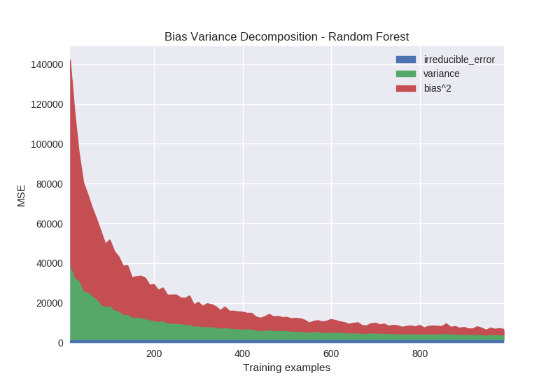
bias variance decomposition random forest training examples graph — Figure 9. Random Forest – Training Examples

Python code specifying models from Figure 9:

model = xgb.XGBRFRegressor(max_depth=12, reg_lambda=0.01)

Conclusions

In conclusion we have learned the following:

Model performance may deteriorate based on two distinct sources of error – bias and variance
Gradient boosting models combat both bias and variance by boosting for many rounds at a low learning rate
The lambda and subsample hyperparameters can also help to combat variance
Random forest models combat both bias and variance via tree depth and number of trees
Random forest trees may need to be much deeper than their gradient boosting counterpart
More data reduces both bias and variance

References

Chen, T., & Guestrin, C. (2016, August). XGBoost: A scalable tree boosting system. In Proceedings of the 22nd acm sigkdd international conference on knowledge discovery and data mining (pp. 785-794). ACM.

Mitchell R, Frank E. (2017) Accelerating the XGBoost algorithm using GPU computing. PeerJ Computer Science 3:e127 https://doi.org/10.7717/peerj-cs.127

Breiman, L. (2001). Random forests. Machine learning, 45(1), 5-32.

Friedman, J. H. (2001). Greedy function approximation: a gradient boosting machine. Annals of statistics, 1189-1232.

Friedman, J. H. (2002). Stochastic gradient boosting. Computational statistics & data analysis, 38(4), 367-378.