DeepStream SDK 3.0 is about seeing beyond pixels. DeepStream exists to make it easier for you to go from raw video data to metadata that can be analyzed for actionable insights. Calibration is a key step in this process, in which the location of objects present in a video stream is translated into real-world geo-coordinates. This post walks through the details of calibration using DeepStream SDK 3.0.
Design
The DeepStream SDK is often used to develop large-scale systems such as intelligent traffic monitoring and smart buildings. This approach to calibration is meant for complex, scalable environments like these, and does not require a physical presence at the site.
Background
One of the big issues with extracting usable data from video streams is taking an object detected by the camera and translating it into a geo-location. Take a traffic camera as an example. When the camera sees a car, the raw image of the car isn’t useful to a smart cities system on its own. The car would ideally be placed in an information grid that also projects a live bird’s eye view of the activities in the city for the operator’s use.
Doing this means translating that camera image into latitude and longitude coordinates corresponding to the car’s location on that intersection. Technically, this is a transformation from the image plane of the camera (image of the car) to a global geo-location (latitude/longitude coordinate). Transformations like this are critical to a variety of use cases beyond simple visualization. Solutions that require multi-camera object tracking, movement summarization, geo-fencing, and other geo-locating for business intelligence and safety can leverage the same technique. We call this calibration.
Let’s take a closer look at how to approach calibration for applications built using DeepStream 3.0.
Approaches to Calibration
Multiple approaches exist for calibrating cameras to yield global coordinates. Several popular methods use a process based on inferring the intrinsic and extrinsic camera parameters. Global coordinates are then inferred with a simple geometric transformation from camera world to the real world.
One way to do this is to use a “checkerboard” pattern to infer the camera parameters. From there, a homomorphic transformation (translation from image plane to real-world) can be used to infer global coordinates.
While the checkerboard approach is a high-fidelity method for calibration, it’s both labor and resource intensive. This makes it impractical for smart cities applications like parking garages and traffic intersections that regularly employ hundreds of cameras in concert. Specifically, the checkerboard approach is:
- Not generalizable. The technique requires creation of custom checkerboards for each application and the checkerboards must be placed at various angles in the camera view.
- Invasive in high traffic areas. Placement of checkerboards requires populated and frequently active areas to be cleared for calibration work, impractical on public roads and in other crowded spaces.
- Not automatable. No uniform or simple way to automate the process exists. Equal time and manpower must be spent on each camera, which can be excessive in some cases.
The approach outlined in this post is suitable for camera systems where cameras are observing a fixed field-of-view (FoV). That is, the cameras are fixed and are all watching the same geo-region. This approach is not suitable for cameras mounted on moving objects (e.g., cars) or Pan-Tilt-Zoom cameras.
Additionally, image size and scaling factors must be the same across all cameras and we must be able to access still images from each camera. We also need access to a global map of the area being watched.
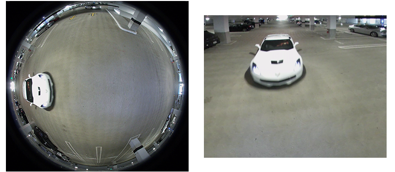
Note that the calibration phase usually involves estimating the camera’s intrinsic and extrinsic parameters, which transforms each pixel into a global location using geometry operations. However, if the camera is a 360-degree camera in several use cases similar to ours, simple transformations may not be possible. The original image from the 360-degree camera has objects appearing in shapes that look distorted. Before we can actually perform the calibration steps, we need to supply pixels from a corrected image.
Consider image (A) in figure 1 below from a 360-degree camera. DeepStream first de-warps the original fisheye image to look like image (B), removing object distortion. This dewarped image is then used for car detection. This undistorted image of the car supplies the pixels for translation into a global coordinate.
![]() System Overview
System Overview
At a high level, this approach constructs corresponding polygons in the camera image and global maps. A transformation matrix maps camera space to global space, as presented in the flow diagram in figure 2.
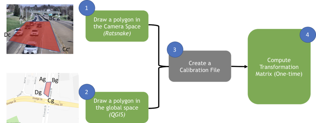
The steps below outline the details on how an application to process this works:
- Draw a polygon on one of the camera images. From this we get four points on a camera plane (eg, points Ac, Bc, Cc and Dc). Use an image annotation tool for this step.
- Draw a corresponding image on the global polygon, resulting in four corresponding points (eg, points Ag, Bg, Cg, Dg). Use a GIS tool for this step.
- Create a CSV file which contains the information required for calibration. For each camera, insert one row which has the information <CameraId, Ac, Bc, Cc, Dc, Ag, Bg, Cg, Dg>”
- Load the CSV file into DeepStream. DeepStream computes a transformation matrix (per-camera) that translates every pixel in the camera plane into global coordinates.
The transformation matrix computes global coordinates for each object detected by the camera.
The Calibration Process
Calibration is a multi-step process, annotating maps, annotating images, and polygon drawing. Let’s walk through the steps:
Annotating Maps
The process involves mapping coordinates in images and global maps. You can use an open source geographical information system tool like QGIS here. QGIS helps you draw polygons and lines with respect to a real map and export the resulting coordinates as a CSV file. You can use this to geo-reference a city block or a parking level image.
Annotating maps requires QGIS. The sources below should help you learn more about installing and using QGIS
- General information about QGIS
- Georeferencer plugin for QGIS: Install Georeferencer plugin into QGIS
- Georeferencing documentation
Annotating Images
There are many image annotation tools available; Ratsnake is a useful, freely available tool. Let’s walk through the steps for annotating images.
Step 1. Capturing image snapshots from cameras
The first step in calibration is obtaining snapshot images from all cameras. Snapshots should show clear, salient feature points of the region of interest. These salient feature points will be mapped to the features seen on a global map. For example, snapshots from cameras installed inside a parking garage should clearly show pillars, parking spot lines painted on the ground, and other features of the building itself. Take the snapshots when the area is empty, or near-empty, to ensure few vehicles, pedestrians, and other large objects block the building features.
We’ll store these snapshots in an directory, and label it for easy reference. For example, make a directory called CAM_IMG_DIR=/mnt/camdata/images/ and save the images there. Individual snapshots may be named with the IP address of the camera they were taken with. For a camera with IP 10.10.10.10, save the snapshot image as ${CAM_IMG_DIR}/10_10_10_10.png.
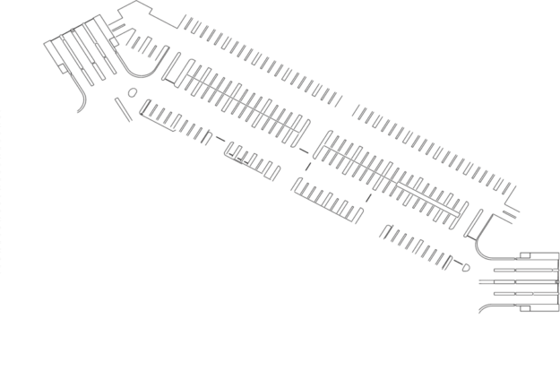
Step 2. Blueprint/CAD image
Download a global map (blueprint or CAD image) of the location being observed — a parking area in our example, as shown in figure 3. Save the map to a directory GIS_DIR (e.g., GIS_DIR==/mnt/camdata/gis/). For example, we save the png file of the parking area as ${GIS_DIR}/parking.png.
Step 3. Georeferencing
Georeferencing maps every point of the region being monitored into a global coordinate system, e.g., latitude and longitude. In other words, it maps every point in the garage to its latitude and longitude.
Depending on the region you are monitoring, you may be able to use existing maps — particularly for outdoor regions. Say you’re using traffic cameras to monitor an intersection. There may well already be a Google or QGIS map you can use to get the coordinates of the intersection and/or traffic light itself.
However, in many use-cases there are no pre-existing georeferenced maps suitable for use in calibration. This is especially true in indoor scenarios, like our parking garage example. That said, you can often find CAD images or blueprints of buildings, and other indoor map files (usually in pdf or picture format) that provide coordinates for at least some key points in the region of interest.
Once you have your CAD image, blueprint, or other indoor map, it’s ready for georeferencing. You do this by placing the blueprint accurately on the global map using QGIS.
Georeferencing works in our methodology if the area in question has at least a few key feature points observable in both the blueprint and the map. Examples might include pillars or corners of staircases.
The process of georeferencing is described below:
- Using a GPS receiver (such as a smartphone), log the latitude and longitude coordinates of various feature points.
- Open the QGIS application. Launch the Georeferencer plugin.
- Open the blueprint (jpg/png image) in the Georeferencer plugin, and follow the guide for georeferencing. Going back to our example from steps 1 and 2 above, if we want to map the parking area, then we use the corresponding png file ${GIS_DIR}/parking.png. Map each of the feature points on both the QGIS map and the blueprint image.
- The resultant output is a georeferenced TIFF file that provides accurate geo-coordinates to any point on the map. Georeferencing yields one image for each blueprint. Save them as ${GIS_DIR}/parking.tif.
Polygon Drawing
Let’s walk through the detailed steps for calibrating one camera (say, camera A with IP 10.10.10.10). Assume that the snap-shots for each camera are stored in ${CAM_IMG _DIR}. We’ll need to repeat these steps for each camera in our set up.
Figure 4 shows the global map and the camera image for camera A.

- Open QGIS and load the global map. In this example, we will load the geo-referenced image of the region covered by camera A. Since this camera covers the above-mentioned parking area, we load the file ${GIS_DIR}/parking.tif.
- Narrow down on the region covered by camera A on the global map. In the above picture, we show the entire global map, and a zoomed in global map on the left-hand side.
- Open the image snapshot ${CAM_IMG_DIR}/10_10_10_10.png using Ratsnake.
- Identify the salient feature points that can be seen on both the global map and the snapshot. In this example, we see pillars and few parking spot lines in the camera image.
- Draw an identifying quadrilateral on the camera image using Ratsnake. Mark the points Ac, Bc, Cc and Dc (see snapshot image on right hand side).
- Draw the same exact quadrilateral on the global map. Call them points Ag, Bg, Cg and Dg. (For details on drawing polygons in QGIS and Ratsnake, see the next section below).
- Note that each point on the global map has to map back to its corresponding point on the snapshot image, i.e. Ag has to map to Ac, and so on. To do this in QGIS, the quadrilateral has to be drawn in the same direction, and starting with the same corresponding point, on both the camera image and in QGIS.
Drawing Polygons in QGIS and Ratsnake
First, let’s go over how to draw a polygon in QGIS. Note the global coordinate for each point on the polygon (e.g. Pt Ag). The global coordinate can take a quadrilateral drawn on the map consisting of four (x,y) points. Each global coordinate (x,y), can be the number of meters from the origin (in x and y direction). The origin may be the center of the building. In addition, the (longitude, latitude) for each point (x,y) is also given. To get the (x,y) from the QGIS tool, follow this procedure:
Drawing the polygons
- Create a new “Vector Layer” in QGIS tool for drawing polygons.
- Add a feature called
CameraId(string) that corresponds to the id of the camera. - Draw the quadrilateral for each camera. Make sure that there are exactly 4 points.
- Update the quadrilateral’s
CameraIdto the camera ID (e.g., “C_10_10_10_10”). - Also, note down the longitude and latitude of the origin point (center of the building).
- Figure 5 shows example polygons that are drawn for an example parking area for various cameras. The background image is the map
(${GIS_DIR}/parking.tif), and the gray boxes are the polygons that have been drawn.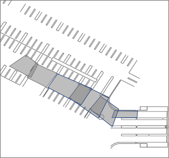
Figure 5. Examples of polygons drawn using QGIS
Get the (longitude, latitude) for each of the polygon points
- Export the vector layer created in the previous step as a CSV. Make sure you have the following columns:
CameraId, longitude0, latitude0, longitude1, latitude1, longitude2, latitude2, longitude3, latitude3 - Read the shapefile and get the attribute of the shape. You may use Python’s
pyshppackage. The documentation shows how to read the latitude and longitude points of the shape, and its attributes (in our caseCameraId) (https://pypi.org/project/pyshp/). The documentation shows how to read the latitude and longitude points of the shape, and its attributes (in our case “CameraId”) - Given an origin point (
longitudeOrigin,latitudeOrigin), convert the latitude and longitude of each shape point to a respective (x, y) based on the distance and angle of the point from the origin. - We will now have four global coordinate points:
(gx0,gy0),(gx1,gy1),(gx2,gy2), and(gx3,gy3)
Draw the polygon on Ratsnake
- Note down the camera coordinates for Ac, Bc, Cc and Dc for each camera. Let us call them as (cx0,cy0), (cx1,cy1), (cx2,cy2), (cx3,cy3). Export these points for each camera.
- Create the Calibration Table (say, as a CSV file nvaisle_2M.csv) similar to the example in table 1 below. This helps DeepStream transform from camera coordinates to global coordinates
| Column | Example | Comments |
| cameraId | C10_10_10_10 | |
| ipaddress | 10.10.10.10 | |
| level | P1 | |
| gx0 | -105.8660603 | Global coordinates |
| gy0 | -12.57717718 | Global coordinates |
| gx1 | -105.9378082 | Global coordinates |
| gy1 | -4.760517508 | Global coordinates |
| gx2 | -96.0054864 | Global coordinates |
| gy2 | -4.86179862 | Global coordinates |
| gx3 | -95.99345216 | Global coordinates |
| gy3 | -11.80735727 | Global coordinates |
| cx0 | 510 | Camera coordinates |
| cy0 | 186 | Camera coordinates |
| cx1 | 1050 | Camera coordinates |
| cy1 | 126 | Camera coordinates |
| cx2 | 1443 | Camera coordinates |
| cy2 | 351 | Camera coordinates |
| cx3 | 21 | Camera coordinates |
| cy3 | 531 | Camera coordinates |
Transferring CSV to DeepStream Server
The CSV create above (nvaisle_2M.csv) file will be added to DeepStream configuration directory, enabling DeepStream to infer the geo-location of detected cars.
The calibration techniques you’ve learned in this post, combined with DeepStream SDK 3.0, enable you to easily create scalable applications with a rich UI to deliver complete situational awareness. Download the DeepStream SDK 3.0 today to get started.