The next-generation 5G New Radio (NR) cellular technology design supports extremely diverse use cases, such as broadband human-oriented communications and time-sensitive applications with ultra-low latency. 5G NR operates on a very broad frequency spectrum (from sub-GHz to 100 GHz). NR employs multiple different OFDM numerologies in physical air interface to enable such diversity, as shown in figure 1 [1]. This contrasts with 4G LTE which uses a single numerology in all cases.

As you can see, the minimum time resolution for scheduling data transmissions is now on ~100 μs time scale [2], about one order of magnitude shorter than LTE, which fixed resolution to 1 ms. Meanwhile, the computational complexity for scheduling further increases in NR since it involves more radio resources (due to greater total bandwidth) and more users per cell compared with LTE. This creates a new technical challenge: how can we design a scheduler for NR that provides optimal scheduling solution while working with the ~100 μs time resolution?
This post introduces a GPU-based Proportional-Fair (PF) scheduler design to address this challenge which we call the “GPF” scheduler. This post presents key ideas from the paper GPF: A GPU-based Design to Achieve ~100 μs Scheduling for 5G NR [3]. Please refer to the paper for more details on the design and complete results.
Timing Requirement for PF Scheduler in 5G
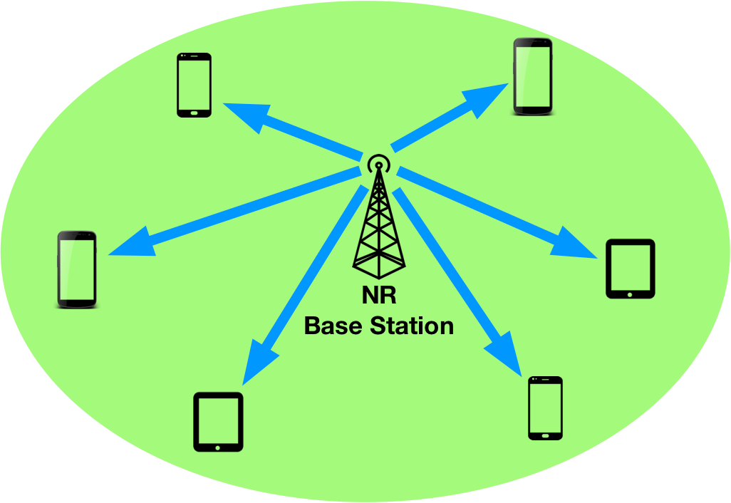
Let’s first look at the Proportional-Fair scheduling problem in an NR cell. We’ll consider the downlink (transmission direction from base station to users) of an NR cell consisting of a base station and a set of users, as shown in Figure 2.
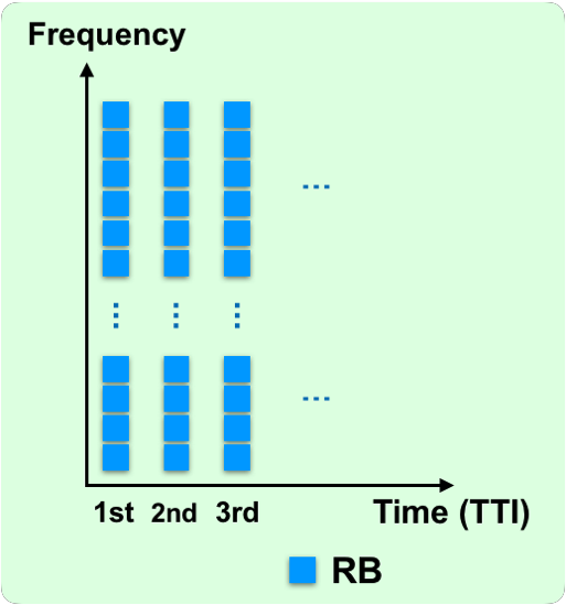
Downlink time and frequency radio resource in this cell is organized as a two-dimensional resource grid, as illustrated in Figure 3. Each small square represents a resource block (RB) spanning 12 OFDM subcarriers in frequency and one Transmission Time Interval (TTI) in time. Under numerology three, the duration of an RB (a TTI) may be as short as 125 μs as shown earlier in Figure 1. The NR scheduler allocates all available RBs in each TTI to users within the cell as one key task. An RB allocates to at most one user while a user can be allocated to multiple RBs. A user’s channel quality varies across RBs due to frequency-selective fading effect, which means that a user’s achieved data rate is different on each RB.
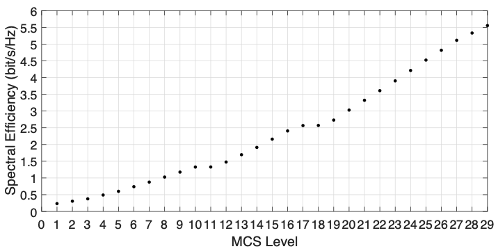
Besides the RB allocation, the scheduler also needs to choose the modulation and coding scheme (MCS) used by each user per TTI. An MCS is a combination of modulation and coding techniques for data transmission. It determines how many bits transmit on an RB for a user. Figure 4 shows that the NR definition includes 29 levels of MCS, each corresponding to a certain spectral efficiency (defined as bits transmitted per Hz per second).
One practical constraint is that each user must employ the same MCS across all resource RBblocks allocated to it in each transmission time interval, due to limited capacity of control signaling channel. What makes the selection of MCS complicated is that for a user, not all MCS levels are feasible on each RB. A higher level of MCS requires better channel quality, and will cause severe bit error on an RB where the channel quality is not good enough. Thus the data rates of a user on its allocated RBs depend on the chosen MCS and the channel quality per RB.
Resource scheduling optimizes with a certain objective. Let’s consider the popular proportional-fairness criterion, achieving a balance between cell throughput and fairness among users. The PF criterion is defined as the sum of log(user k’s long-term average data rate) over all users k=1, 2, 3, … in the cell. In each TTI, the scheduler jointly allocates RBs and selects MCS per user with the objective of maximizing PF criterion.
Proof exists that this problem is NP-hard. Any practical NR network setting will find it challenging to discover a near-optimal scheduling solution within a TTI’s duration, which will be as short as 125 μs. In fact, none of existing PF schedulers designed for 4G LTE can achieve this goal. A major reason is that these LTE PF schedulers are all of sequential designs that need to go through a large number of iterations to find solution.
GPF – A Novel GPU-based PF Scheduler
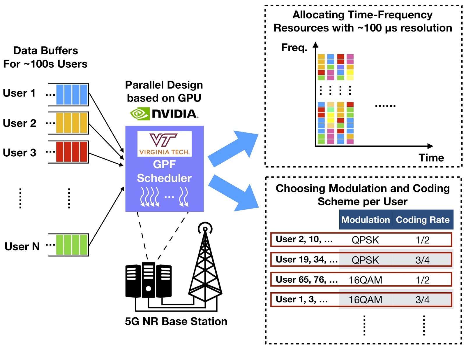
How does GPF manage to meet the ~100 μs real-time requirement? Let’s examine its GPU-based parallel design. An illustration of the system architecture is given in Figure 5. GPF determines the RB allocation and MCS selection for each user with input of each user’s channel quality across all RBs in each TTI. Maximizing the PF criterion as defined above is the main goal of GPF.
We tailored GPF for implementing on GPUs. The basic idea: find scheduling solutions through solving a certain number of small and independent sub-problems on the GPU in parallel. The solution to each sub-problem is a feasible solution to the original PF scheduling problem. The output solution of GPF is then the best one among all sub-problem solutions. So what does a sub-problem look like?
Let’s define sub-problems. Assume the choice of MCS is fixed for each user (1 out of the 29 levels per user). How are RBs allocated to maximize the PF objective? This problem is much simpler than the original problem and can be solved exactly and efficiently. However, the total number of possible MCS choices for all users is astronomical when the user population is large For example, 100 users in the cell generates 29100 possible sub-problems.
Fortunately, not all sub-problems are actually worth solving. What MCS levels are more likely chosen for a specific user in an optimal scheduling solution? Observing a large number of optimal solutions yields a high (empirical) probability for each user to only use their highest several levels of MCS feasible on some RBs.
For example, assume User 1’s downlink channel can support MCS 1, 2, …, 23 (i.e., MCS levels beyond 23 are infeasible on all RBs, MCS 23 is feasible on a few RBs, MCS 22 is feasible on a bit more RBs, and so forth). The optimal solution for User 1 would be to assign him to MCS 21, 22, or 23. This effect validates through an empirical and statistical approach as described in Section 5.3 in [3]. Since there are many users in the cell, maximizing PF objective means each user should allocate to RBs where its channel quality is good and thus high MCS levels are feasible.
Thus, the first step to reduce the number of sub-problems we actually solve on GPUs is limiting the MCS choices per user to a subset containing only the highest several levels of feasible MCS. We call this step “intensification”, meaning that we are intensifying our search of solution on a promising sub-space of the original problem space. Here we use a variable d to control the number of considered MCS levels (descending from the highest feasible one), which is common to all users. The optimal value of d depends on the user population size and can be determined by an off-line empirical approach as described in [3]. Our results show that d should be set to 6, 3, 3 and 2 for 25, 50, 75 and 100 users per cell, respectively.
Although intensification significantly reduces the number of sub-problems we need to consider, the promising sub-space is still too large for any d>1. In other words, for d=2 and 100 users per cell, we have 2100 remaining sub-problems. Therefore, the second step is to select a number K of sub-problems from the promising sub-space via random sampling subject to uniform distribution (i.e., for each user, choose each MCS within the promising subset with a probability 1/d). The value of K should be set based on the computational capability of the GPU. We sample K=300 sub-problems in each TTI when using an NVIDIA Quadro P6000 GPU used for these experiments.
Figure 7 highlights the actual implementation on GPU. We use a one-dimensional grid of 30 thread blocks to generate and solve 300 sub-problems, with each block addressing 10 sub-problems. When the best sub-problem solution from each block is found, we use another thread block to find the best output scheduling solution. For more details about the implementation, please refer to Section 6 in [3].

Achieving Near-Optimal Performance
Since we only consider K out of 29N (N is the number of users per cell) sub-problems in each TTI, can we find a near-optimal scheduling solution? The answer is yes. Although each sub-problem solution only has a small probability to be near-optimal, we will have a high probability of achieving near-optimality when K is practically large (e.g., for K=300).
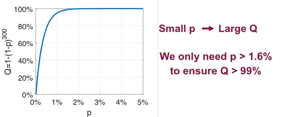
To see this, let’s denote p as the probability of each sub-problem solution being near-optimal (e.g. 99%-optimal), and Q=1-(1-p)K as the probability of having at least 1 out of K sub-problem solutions being near-optimal. The relation between p and Q when K=300 is shown in figure 7. We can see that a small p is enough to ensure a large Q (e.g., p>1.6% ensures Q>99%). Experiments for N=100 users revealed that each sub-problem has a probability p=3.0% to achieve 99.5%-optimality. This implies with K=300 sub-problems we can achieve 99.5%-optimality with a high confidence factor with probability Q=99.99%.
Meeting Timing Requirement
We implemented GPF with an Nvidia Quadro P6000 GPU to validate performance. Figure 8 shows GPF’s performance with 100 available RBs per TTI and N=25, 50, 75 and 100 users. We can see that GPF can achieve near-optimal PF objective while meeting the ~100 μs requirement on computational time.

Conclusion
This post presents GPF, the world’s first successful PF scheduler capable of meeting the ∼100 µs time requirement for 5G NR. The design of GPF is based on a novel decomposition of the original PF scheduling problem into a large number of small and independent sub-problems. Employing intensification and random sampling techniques enables selecting a subset of sub-problems in each TTI to match the computational capability of a GPU. Extensive experiments on an Nvidia Quadro P6000 GPU on a desktop Dell computer show that GPF can achieve near-optimal performance while meeting the ∼100 µs time requirement.
Acknowledgment
This research was supported in part by the National Science Foundation.
References
[1] 3GPP TS 38.211 version 15.4.0, Physical channels and modulation
[2] 3GPP TR 38.804 version 14.0.0, Study on New Radio access technology; Radio interface protocol aspects
[3] Y. Huang, S. Li, Y. Thomas Hou, and W. Lou, “GPF: A GPU-based Design to Achieve ~100 μs Scheduling for 5G NR,” in Proc. ACM MobiCom 2018, pp. 207-222, Oct. 29-Nov. 2, 2018, New Delhi, India.