Sign up for the latest Speech AI news from NVIDIA.
Conversational AI is the technology that allows us to communicate with machines like with other people. With the advent of sophisticated deep learning models, the human-machine communication has risen to unprecedented levels. However, these models are compute intensive, and hence require optimized code for flawless interaction. In this post, we’ll walk through how to convert a PyTorch model through ONNX intermediate representation to TensorRT 7 to speed up inference in one of the parts of Conversational AI – Speech Synthesis.
Conversational AI
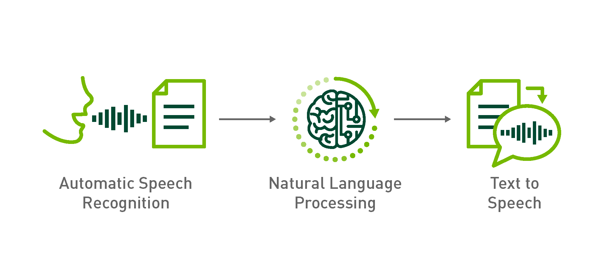
A typical modern Conversational AI system comprises 1) an Automatic Speech Recognition (ASR) model, 2) a Natural Language Processing model (NLP) for Question Answering (QA) tasks, and 3) a Text-to-Speech (TTS) or Speech Synthesis network. A recently published technical blog describes how you can build domain specific ASR models on GPUs.
A challenge for Conversational AI is that in order for the conversation to be natural, the machine has to respond promptly to human actions. When you talk with friends, their reactions to your comments or questions are instantaneous, and you probably expect similar responsiveness from the devices you use. This is challenging, since sequential signals such as waveform are difficult to parallelize during inference. This is the case for many of the state-of-the-art neural networks, including Tacotron 21, that use the aforementioned recurrent layers, or operate in an autoregressive manner, where the output signal is fed back to the input.
The utterances we speak and hear are sequential signals of varying duration. In the context of neural network applications, we define the variability of utterance length as variable-size input/output. A conversational AI system has to correctly handle this variability both on the system level and model level, and in the latter it typically processes the signals using recurrent layers, such as Long Short-Term Memory (LSTM) units.
TensorRT for Conversational AI
NVIDIA TensorRT is an SDK for high-performance deep learning inference. It includes a deep learning inference compiler and runtime that delivers low latency and high-throughput for deep learning inference applications.
TensorRT 7 can compile recurrent neural networks to accelerate for inference. It has new APIs for supporting the creation of Loops and recurrence operations with batched inputs. TensorRT 7 also includes an updated ONNX parser that has complete support for dynamic shapes, i.e., defer specifying some or all tensor dimensions until runtime. Support for recurrent operators in the ONNX opset, such as LSTM, GRU, RNN, Scan, and Loop, has also been introduced in TensorRT 7 – enabling users to now import corresponding operations from Tensorflow and PyTorch into TensorRT via the ONNX workflow. Operations such as RandomUniform (generate random uniform distribution), and Expand (expand tensors) are used to introduce variance in our implementation of Tacotron 2. Other operator additions of interest in this release include – tensor creation and manipulation operations (ConstantOfShape, Tile), Boolean operations (Where, Equal, Not, Less, Greater, And), Casting and ElementWise operations (Erf). For a complete list of new features, refer to the TensorRT Release Notes.
TensorRT 7 has a new and flexible way to represent recurrences in a network and allows a variety of layers within a recurrence. A set of important performance optimizations has been constructed based on this enhanced internal representation. A recurrence layer resembles a traditional programming language loop structure, which calls for well-known and new loop-nest optimizations. An innovative “time fusion” optimization fuses the instances of layer (or input) GEMM inside an LSTM layer across the timesteps to fully utilize machine resources with or without explicit loop unrolling. Loop invariant code motion moves computations, which are invariant to loop iterations, outside a loop to avoid redundant computations. An incorporated linear algebra fusion examines data mapping and fuses not only point-wise layers, but also reduction layers and data movement layers, e.g. transpose, concat, split, etc. General RNNs may have multiple sets of weights feeding to different cells, and TensorRT 7 is able to concatenate them once at load time in a way tailored toward fused GEMM layers without incurring expensive runtime concatenation.
In this blog post, we will focus on the Text-to-Speech part of the conversational pipeline, specifically running Tacotron21 and WaveGlow2 in TensorRT 7. In TTS, the input text is converted to an audio waveform that is used as the response to user’s action. Both models require dynamic shapes: Tacotron 2 consumes variable-length-text and produces a variable number of mel spectrograms, and WaveGlow processes these mel-spectrograms to generate audio. The Encoder and Decoder parts in Tacotron 2 use LSTM layers. RandomUniform operation allows us to introduce variance in the output spectrograms by emulating dropouts during inference.
Speech Synthesis with Tacotron 2 and WaveGlow
In our previous post, you could learn about the architecture of the TTS system and performance in the native PyTorch framework with the support of Automatic Mixed Precision from APEX. Here, I’d like to focus on the networks’ structure as it is implemented in PyTorch, since this is our starting point for deploying the models on TensorRT 7.
Tacotron 2
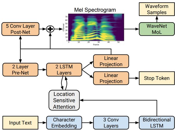
Tacotron2 is a sequence-to-sequence model with attention that takes text as input and produces mel spectrograms on the output. The mel spectrograms are then processed by an external model—in our case WaveGlow—to generate the final audio sample.
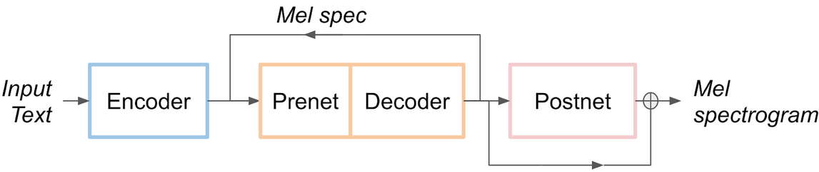
For the purpose of this blog, we can simplify the model into the following diagram, where we group the elements into Encoder, Decoder and Postnet. The Decoder is autoregressive: in each iteration of Python while loop, it outputs a mel spectrogram that is fed back to its input. The loop stops when a given threshold for the stop token is reached. Both the Encoder and Decoder use LSTM layers.
The Decoder loop operates in the following manner in the PyTorch code:
while True:
    decoder_inputs = (self.prenet(decoder_input), ...)
    decoder_outputs = self.decode(decoder_inputs)
    gate_output = decoder_outputs[1]
    if sigmoid(gate_output) > gate_threshold:
        break
    decoder_input = decoder_outputs[0]
The structure in Figure 3 suggests splitting the Tacotron 2 model into three parts and exporting them separately as three TensorRT engines with the Prenet+Decoder (from now on we’ll just call it Decoder) engine running in a Python loop, just as I’ve done in the PyTorch code above. We will also put the last addition of the residual into the Postnet engine.
So let’s get started with the export workflow, in which we will first convert the model to ONNX IR and from this build the TensorRT engine. As a basis for our export, we use the model from NVIDIA’s Deep Learning Examples on GitHub. You can obtain trained checkpoint for Tacotron 2 from the NGC models repository.
For the export, we have to modify the Tacotron 2 model in a few places. First, we will put the memory layer from the Decoder inside the Encoder, as it has to be used only once per utterance. Furthermore, the Tacotron 2 code uses LSTMCells which have just one layer. For the export, we need to replace LSTMCells in attention_rnn and decoder_rnn layers with regular LSTMs, since only the latter is supported by ONNX.
We first define the attention_rnn layer as:
self.attention_rnn = nn.LSTM(dec.prenet_dim +
                             dec.encoder_embedding_dim,
                             dec.attention_rnn_dim, 1)
And in the decode method, we replace the following code:
attention_hidden, attention_cell = self.attention_rnn(
            cell_input, (attention_hidden, attention_cell))
With code that additionally has to take care of input and output dimensions:
_, (attention_hidden_res, attention_cell_res) = self.attention_rnn(
            cell_input.unsqueeze(0), (attention_hidden.unsqueeze(0),
                                      attention_cell.unsqueeze(0)))
attention_hidden = attention_hidden_res.squeeze(0)
attention_cell = attention_cell_res.squeeze(0)
We treat decoder_rnn similarly. Since we want to use checkpoints produced with the scripts from the original repository, we also need to manually load weights from the LSTMCells:
def lstmcell2lstm_params(lstm, lstmcell):
    lstm.weight_ih_l0 = torch.nn.Parameter(lstmcell.weight_ih)
    lstm.weight_hh_l0 = torch.nn.Parameter(lstmcell.weight_hh)
    lstm.bias_ih_l0 = torch.nn.Parameter(lstmcell.bias_ih)
    lstm.bias_hh_l0 = torch.nn.Parameter(lstmcell.bias_hh)
Unlike most of neural network models, Tacotron 2 uses dropouts during inference to introduce variance in the output signal. To have dropouts in the engine, I implemented it myself:
def prenet_infer(self, x):
    z = torch.zeros(1, dtype=torch.float32).cuda()
    for linear in self.layers:
        x = F.relu(linear(x))
        x0 = x[0].unsqueeze(0)
        mask = torch.le(torch.rand(256, device='cuda').to(torch.float32), z).to(torch.float32)
        mask = mask.expand(x.size(0), x.size(1))
        x = x*mask*2.0
    return x
Notice that we benefit from the addition of RandomUniform in the form of rand() function in TensorRT 7. There are a few other modifications in the code that deal with the Encoder and Postnet – you can inspect them in the Tacotron 2 export script.
WaveGlow
The WaveGlow model is a flow-based generative model that generates audio samples from Gaussian distribution using mel spectrogram conditioning.
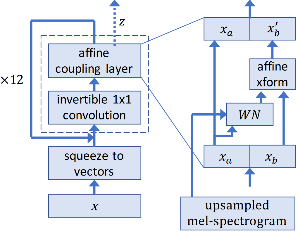
Also for the WaveGlow model you can obtain the trained checkpoint from the NGC models repository. In this model, we need to change the 1D convolutions to 2D convolutions with the second kernel dimension set to 1.
def convert_conv_1d_to_2d(conv1d):
    conv2d = torch.nn.Conv2d(conv1d.weight.size(1),
                             conv1d.weight.size(0),
                             (conv1d.weight.size(2), 1),                             stride=(conv1d.stride[0], 1),
                             dilation=(conv1d.dilation[0], 1),
                             padding=(conv1d.padding[0], 0))
    conv2d.weight.data[:,:,:,0] = conv1d.weight.data
    conv2d.bias.data = conv1d.bias.data
    return conv2d
We also need to take care of the inverse initialization in the Invertible1x1Conv layer. In the PyTorch code, this is done on the fly when the inference is run for the first time. For proper ONNX export, we have to run the initial inference in PyTorch so that the inverse gets initialized. Moreover, we need to take care of converting this inverse to 2D convolution:
def convert_convinv_1d_to_2d(convinv):
    conv2d = torch.nn.Conv2d(convinv.W_inverse.size(1),
                             convinv.W_inverse.size(0),
                             1, bias=False)
    conv2d.weight.data[:,:,:,0] = convinv.W_inverse.data
    return conv2d
There are a few other modifications in the code that deal with the WaveGlow model – you can inspect them in the WaveGlow export script.
Exporting Models to TensorRT through ONNX
Now comes the most exciting part – getting the models to run in TensorRT 7! We first export the models to ONNX Intermediate Representation (IR), which is then consumed by the TensorRT ONNX parser. Shown below are the steps for exporting the decoder model to ONNX, and the other 2 components are exported in a similar fashion.
torch.onnx.export(decoder_iter, dummy_input, "decoder_iter.onnx",
                  opset_version=opset_version,
                  do_constant_folding=True,
                  input_names=["decoder_input", "attention_hidden",
                               # a few more elements
                               "Processed_memory", "mask"],
                  output_names=["decoder_output", "gate_prediction",
                                # a few more elements
                                "out_attention_context"],
                  dynamic_axes={"decoder_input" : {0: "batch_size"},
                                "attention_weights" : {0: "batch_size", 1: "seq_len"},
                                # a few more elements
                                "out_attention_context" : {0: "batch_size"}})
The list of input and output names is quite long, since we need to spell out all variables with dynamic shapes. We have specified the names of inputs and outputs in the lists input_names and output_names, respectively. We use constant_folding=True to precompute constants in the model. To build all the engines from their respective ONNX IRs, we use this script:
def build_engine(model_file, shapes, max_ws=512*1024*1024, fp16=False):
    TRT_LOGGER = trt.Logger(trt.Logger.WARNING)
    builder = trt.Builder(TRT_LOGGER)
    builder.fp16_mode = fp16
    config = builder.create_builder_config()
    config.max_workspace_size = max_ws
    if fp16:
        config.flags |= 1 << int(trt.BuilderFlag.FP16)
    profile = builder.create_optimization_profile()
    for s in shapes:
        profile.set_shape(s['name'], min=s['min'], opt=s['opt'], max=s['max'])
    config.add_optimization_profile(profile)
    explicit_batch = 1 << (int)(trt.NetworkDefinitionCreationFlag.EXPLICIT_BATCH)
    network = builder.create_network(explicit_batch)
    with trt.OnnxParser(network, TRT_LOGGER) as parser:
        with open(model_file, 'rb') as model:
            parsed = parser.parse(model.read())
            engine = builder.build_engine(network, config=config)
            return engine
Notice the profile.set_shape() function – TRT can efficiently optimize inference code for the minimum, maximum and optimal input sizes. We also use trt.OnnxParser that parses our previously generated model representations. To run the inference with TRT, we use run_trt_engine function that accepts engine context, the engine itself, and input and output tensors as a dictionary.
def run_trt_engine(context, engine, tensors):
    bindings = [None]*engine.num_bindings
    for name in tensors.keys():
        idx = engine.get_binding_index(name)
        tensor = tensors.get(name)
        bindings[idx] = tensor.data_ptr()
        if engine.is_shape_binding(idx) and is_shape_dynamic(context.get_shape(idx)):
            context.set_shape_input(idx, tensor)
        elif is_shape_dynamic(context.get_binding_shape(idx)):
            context.set_binding_shape(idx, tensor.shape)
    context.execute_v2(bindings=bindings)
In our inference script, we first setup the dictionary with tensor names and tensors themselves:
init_decoder_tensors(decoder_inputs, decoder_outputs):
    decoder_tensors = {
        # inputs
        'decoder_input': decoder_inputs[0],
        'attention_hidden': decoder_inputs[1],
        # ...
        # outputs
        'out_attention_hidden': decoder_outputs[0],
        'out_attention_cell': decoder_outputs[1],
        # ...
    }
Afterwards, we pass them to the engine:
decoder_context = decoder_iter.create_execution_context()
    while True:
        decoder_tensors = init_decoder_tensors(decoder_inputs, decoder_outputs)
        run_trt_engine(decoder_context, decoder_iter, decoder_tensors)
        # [...]
The order of output bindings in a TensorRT engine is not determined by the order of definition in the ONNX export, but rather by the order of creation within the engine. By passing the inputs and outputs as dictionary, we are sure that the bindings are chosen correctly (we must also remember that the input and output names have to be unique). We provide full code for Tacotron 2 and WaveGlow inference in the TensorRT inference script.
Benefits of Using TensorRT 7
Table 1 below shows inference results for end-to-end inference with Tacotron 2 and WaveGlow models. The WaveGlow model has 256 residual channels. The results were gathered from 1,000 inference runs on a single NVIDIA T4 GPU. Latency is measured from the start of Tacotron2 inference to the end of WaveGlow inference. Throughput is measured as the number of generated audio samples per second. RTF is the real-time factor which tells how many seconds of speech are generated in 1 second of wall time. For a real-time application, you need to achieve an RTF greater than 1. We can achieve RTF of 6.2 using TensorRT 7, which is 13 times faster than CPU1.
| Framework | Batch size | Input Length | Precision | Avg Latency (s) | Avg RTF | Speed-up vs CPU |
| PyTorch+
TensorRT |
1 | 128 | mixed precision | 1.14 | 6.20 | 13x |
| PyTorch (T4) | 1 | 128 | mixed precision | 1.63 | 4.30 | 9x |
| PyTorch CPU | 1 | 128 | FP32 | 14.13 | 0.48 | 1x |
Table 1: Comparison of PyTorch and TensorRT TTS inference latencies on 1xNVIDIA T4 GPU
What’s Next?
In this post, we showed how to export a PyTorch model to TensorRT 7 for inference. In the presented scripts I still used PyTorch, since it allowed smooth transition to TensorRT API. If you don’t want to be dependent on any deep learning framework, you can switch to PyCUDA for managing inputs and outputs of the TensorRT engines. Moreover, for even more optimized code, you can switch from Python to C++ API in TensorRT.
You can try Text-to-Speech in TensorRT yourself by following the TensorRT Readme in Deep Learning Examples.
1 CPU-only specifications: Intel Xeon E5-2698 v4, PyTorch-19.06-py3 NGC. GPU-server specification: Gold 6240@2GHz 3.9GHz Turbo (Cascade Lake) HT On, T4 16GB, PyTorch-19.11-py3 NGC
References
- [Shen et al 2018] “Natural TTS Synthesis by Conditioning WaveNet on Mel Spectrogram Predictions” Jonathan Shen, Ruoming Pang, Ron J. Weiss, Mike
- [Prenger et al 2018] “WaveGlow: A Flow-based Generative Network for Speech Synthesis” Ryan Prenger, Rafael Valle, Bryan Catanzaro
- Tacotron 2 and WaveGlow inference scripts
- TensorRT Release Notes