Implementing Stochastic Levels of Detail with Microsoft DirectX Raytracing

Level-of-detail (LOD) refers to replacing high-resolution meshes with lower-resolution meshes in the distance, where details may not be significant. This technique can help reduce memory footprint and geometric aliasing. Most importantly, it has long been used to improve rasterization performance in games. But does that apply equally to ray tracing?

The render time for rasterization is $O(N)$ , where $N$ is the number of triangles, whereas the render time for ray tracing is significantly better at $O(log N)$ . So, you would expect LOD to be less critical for ray tracing, but perhaps it can still provide worthwhile performance improvements.

In this post, we explore this question. In addition, we demonstrate one possible way to implement stochastic LOD using the Microsoft DirectX Raytracing (DXR) API. We assume that you have a basic familiarity with DXR. For more information, see the following resources:

Introduction to NVIDIA RTX and DirectX Ray Tracing
DX12 Ray Tracing Tutorial Part 1
DirectX Raytracing (DXR) Functional Spec (Microsoft)
D3D12 Raytracing Samples (Microsoft)

Figure 1. Screenshot from the DXR sample provided with this post. LODs are beneficial in open scenes like this with large depth ranges. Color indicates the LOD level. The most distant models are rendered with 128 times fewer triangles than the closest ones (eight LODs, 2x reduction in triangle count between each level).

Stochastic LODs

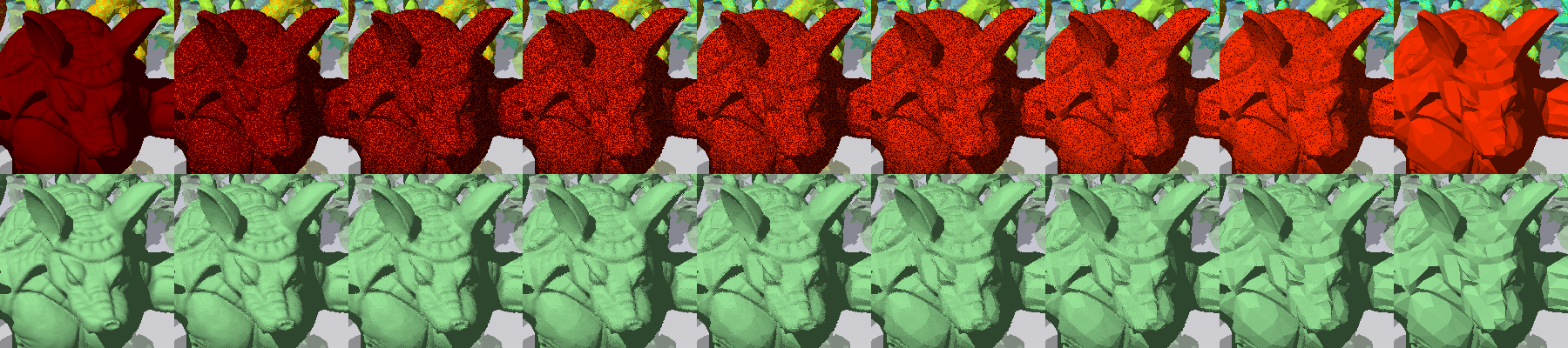
Stochastic LOD is the primary technique used by games to create smoother transitions between LODs. For example, in Unreal Engine 4, stochastic LOD is called Dithered LOD Transitions. Without stochastic techniques, the abrupt, discrete transition between LODs can result in distracting “popping” artifacts where an object suddenly shifts in appearance. Stochastic LOD creates a cross-dissolve between LOD levels by randomly assigning pixels to either the closer or farther LOD (Figure 2). For more information, see the Finding Next Gen: CryEngine 2. SIGGRAPH Advanced Real-Time Rendering in 3D Graphics and Games course, pp. 97-121.

Picture shows the transition from a higher LOD to lower LOD, with color encoding and without. — *Figure 2*. Stochastic LOD with eight steps of transition with color encoding (top row) and without (bottom row). The transition has been exaggerated (64x reduction in triangle count) for this figure to make it easier to see the transition. Click image to enlarge.

LOD in DXR

To implement discrete LOD transitions, we choose one LOD to use for each object, based on its distance to the camera. Objects further away use lower-resolution meshes, and close-by objects use higher resolution.

In our sample, we use the depth of the object in camera space to compute an LOD parameter, $l$ . $l$ varies continuously from 0 at a depth $z_n$ to $L$ at depth $z_f$ , where $L$ is the number of LODs for an object. $z_n$ and $z_f$ are chosen based on the characteristics of a given scene, much like the near and far distances for the depth buffer in rasterization. For more information about computing the LOD parameter, see the ChooseLod function in the sample code. The LOD parameter for a given object is then used directly to select its mesh.

Because the LOD parameter changes as the camera or objects move, we must recompute the LOD parameter for each object every frame. We then rebuild the top-level acceleration structure (TLAS) with updated pointers to the correct mesh LODs. Games typically rebuild the TLAS every frame to handle dynamic objects, so this rebuild does not incur any additional overhead.

Secondary rays and LOD

Most ray tracing–enabled games use the discrete LOD approach described earlier because it is both straightforward and effective. Critically, it also matches the LOD selection behavior of rasterization passes in many hybrid renderers. Hybrid rendering is a common method in games, where a G-Buffer with primary hit data is generated using traditional raster methods, and a subsequent ray tracing pass uses that data as a starting point to compute secondary effects, such as reflections or shadows.

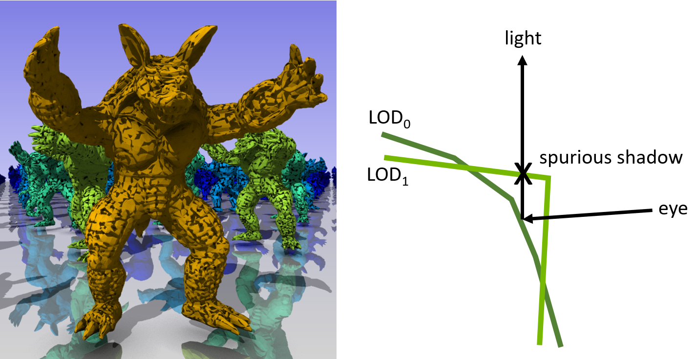
Whether primary hits are produced by a rasterization pass or by ray tracing, this is an important thing to keep in mind: Any secondary ray starting from a primary hit must “see” the same LODs for objects as the primary ray (or rasterizer) did. Failure to guarantee this means that secondary rays might miss intersections or find spurious hits due to the mismatch in scene representations between the primary and secondary rays (Figure 3). This in turn can lead to visual artifacts like light leaks, objects disappearing in reflections, or incorrectly shadowed areas.

It is not sufficient for primary and secondary rays to agree on the LOD level of the object hit by the primary ray. Other unrelated objects may be close enough to the primary hit point to cause the previously mentioned robustness issues as well, so these objects must be consistent too. The problem is also not limited to the transition from primary to secondary rays. It applies to higher-level bounces as well, for example, reflections of reflections, multi-bounce global illumination, and so on.

Example of shadow artifacts and a diagram showing how they occur. — *Figure 3*. Spurious shadows resulting from using a higher LOD for primary rays (LOD₀) and lower LOD for secondary rays (LOD₁).

That said, under some circumstances it may be beneficial and acceptable for applications to knowingly violate the principle that all rays along a path should see the same LODs. For example, you could imagine tracing a short—and therefore relatively cheap—secondary ray against a high-detail representation of the scene. If that short ray misses, you would trace another, longer ray starting at the end point of the first ray, but against a much lower detail version of the scene.

Depending on various factors, like the threshold distance between the short and the long ray and the difference in scene detail, this method may pay off in terms of performance. However, because the scene LODs change between the short and the long ray, the application has to accept the possibility of invalid or missed intersections. The idea is therefore feasible only for situations where a certain error may be acceptable, for example very diffuse effects or higher-level light bounces. We did not explore this path in this post, but wanted to highlight it as a starting point for further experiments.

Stochastic LOD transitions

For stochastic LOD transitions, an object can be in an intermediate state transitioning between two LODs. We include both LODs in the TLAS, but we need a way to choose which of the two LODs to intersect for each pixel. Furthermore, that choice needs to happen independently per object, because different objects may be at different points within an LOD transition.

DXR supports specifying an 8-bit instance mask at TLAS build, which is then combined with a per-ray mask to determine whether an instance should be tested for intersection or ignored. Specifically, the two masks are ANDed together. If the result is zero, the instance is ignored. We use this instance mask feature to stochastically select between two adjacent LODs.

Transition interval

$k_a = \min(0,\lfloor l \rfloor)$ and $k_b = \max(\lceil l \rceil, L-1)$ give the indices of the LODs on either side of the transition, and the fractional part of $l$ , $f = l - \lfloor l \rfloor$ gives the degree of transition between them.

In practice, you may want the transition to occur over a shorter interval. If you parameterize the transition interval by $t \in [0,1]$ , where 0 means that there is no transition interval, just a discrete step from one level to next, and 1 means that the transition happens over the entire range for one LOD, then you can modify $f$ to be $f' = \mathrm{clamp}((f - 0.5)/t + 0.5, 0, 1)$ .

Figure 4 shows $f'$ for various values of $t$ .

Three graphs showing the transition intervals 0.2, 0.5, and 1.0. — *Figure 4.* *Remapping the fractional part of the LOD parameter to shorten the duration of the transition*, $t$ , *from one LOD to the next*.

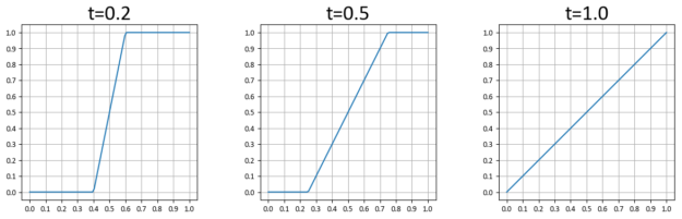*Figure 4.* *Remapping the fractional part of the LOD parameter to shorten the duration of the transition*, $t$ , *from one LOD to the next*.

Setting the instance masks

We initialized the instance masks such that setting a single random bit in the per-ray mask results in the desired cross-dissolve effect. For each object, we needed two instances, one for LOD $k_a$ and the other for $k_b$ . We set the number of bits (8 total) in the instance mask for $k_b$ proportional to the degree of transition $f'$ . The degree of transition for $k_a$ is $1 - f'$ . We set the instance mask for $k_a$ by complementing the mask for $k_b$ .

The code looks something like the following:

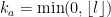
maskB = (1 << int((8 + 1)*f_prime) ) - 1;
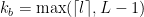
maskA = (~maskB) & 0xFF;

When calling TraceRay in the ray generation shader, we set the 8-bit ray mask to a single uniformly random bit. This selects $k_a$ or $k_b$ according to their respective degree of transition. Because neighboring rays are likely to use different random ray masks, this results in the desired stochastic transition effect.

Propagating the ray mask along a path

As discussed earlier, when tracing paths with multiple bounces, it is important that subsequent rays in a path see the same LODs. To achieve this with our stochastic approach, we use the same ray mask for each ray along a path. DXR does not have a way to query the current ray mask so we propagate it to closest-hit shaders using the ray payload.

Limitations

Our implementation of stochastic LOD is fully hardware-accelerated on NVIDIA RTX GPUs, but there are several limitations. One limitation is that the instance and ray masks only consist of 8 bits, which means that we only get eight levels for stochastic LOD transitions (Figure 2). This is more apparent the slower the movement and the wider the transition intervals between LODs.

Another limitation is that using the instance and ray masks for stochastic LOD makes them unavailable for other uses, like enabling or disabling certain groups of geometry. It is sometimes possible to partition the mask bits to accommodate different use cases, but this further reduces the number of transition levels.

Stochastic LOD also suffers some performance penalties relative to discrete LOD. Stochastic LOD, in general, increases GPU warp divergence due to adjacent pixels tracing against different objects. Our implementation of stochastic LOD also doubles the number of instances in the TLAS, which slightly increases TLAS build time.

Stochastic LOD example

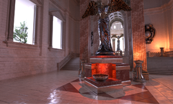
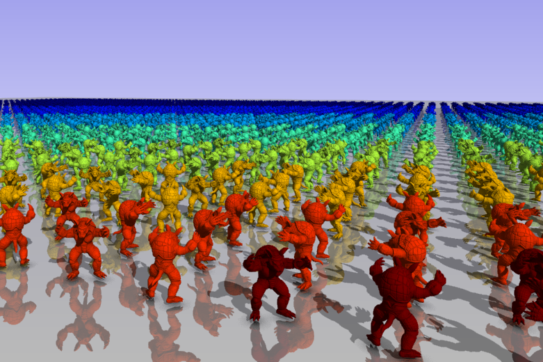
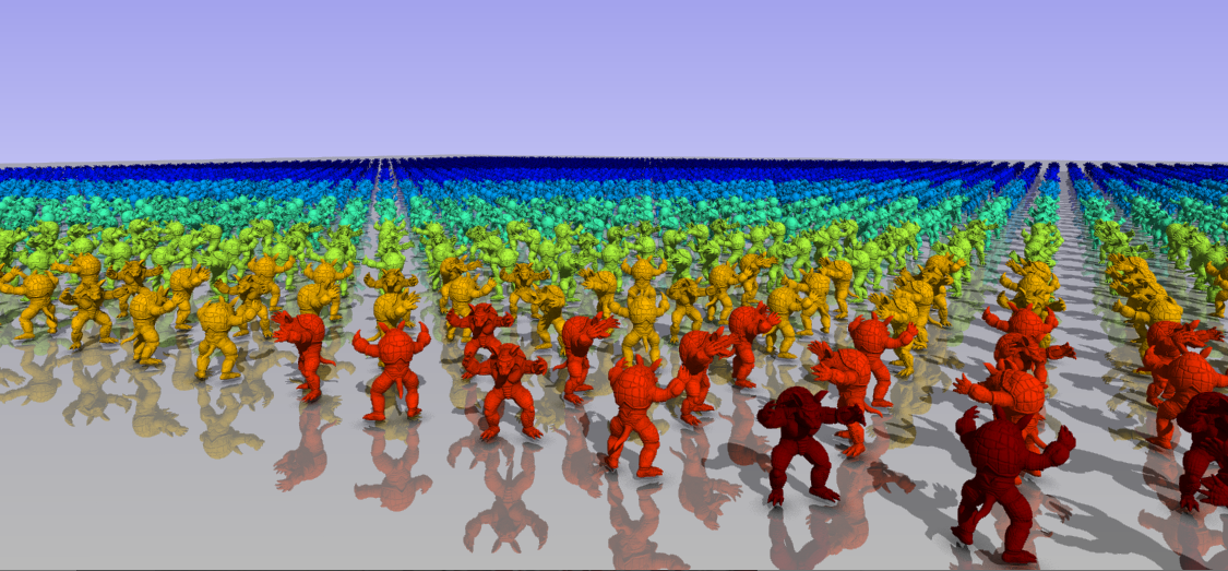
Figure 1 shows a screenshot from the sample code included with this post. We implemented ray traced reflections, shadows, and ambient occlusion.

The objects in the scene are colored according to their LOD, with the highest LOD as red and the lowest LOD as blue. The scene itself consists of several instanced armadillo models. We build a bottom-level acceleration structure (BLAS) for each LOD of the model. The TLAS is built from randomly rotated instances that reference the BLAS for the selected LOD.

The LOD parameters can be tweaked with several settings. The LOD range ( $z_n$ and $z_f$ ) are given in normalized coordinates where a value of 1 represents the radius of the entire scene. The LOD bias offsets the computed LOD parameter.

When the camera is still, frames are accumulated into the output to provide antialiasing. Each subframe gets its own random seed. Over multiple frames, the accumulation of stochastic LOD produces a blend between the two LODs. To better see the effect of stochastic LOD, pause the subframes. To see the individual transition levels, expand the transition interval to 1 and move the LOD bias slider slowly. This is how we created Figure 2.

The LOD meshes used in the sample were generated with QSlim, a command-line utility that reduces an input mesh in OBJ format to a specified number of triangles. You may want to use QSlim to experiment with your own models.

Implementation details

Most of the sample code is straightforward DirectX 12. We started the code from the DX12 Ray Tracing Tutorial Part 1, but retained only a few helper classes for the layout of the shader binding table and to create the state object for the ray tracing pipeline.

The LOD selection step is performed on the GPU. For simplicity, we implemented it using a ray generation shader rather than a compute shader. This avoids the need to set up another pipeline state object. Because some parameters are shared between LOD selection and rendering, we placed all the parameters in a common constant buffer.

The LOD selection shader fills an array of instance descriptors on the device, which are then used to build the TLAS. The relevant C++ struct D3D12_RAYTRACING_INSTANCE_DESC uses several bit-fields. HLSL does not support bit-fields, so you have to pack the fields into uints manually.

Performance

To evaluate performance, we included two benchmarking modes that can be invoked by pressing the following number keys:

1: Sweep through several predefined views.
2: Sweep through the range of transition intervals.

Figure 5 shows the views for the first mode. The first view is from an aerial perspective over the whole scene. The subsequent views are at increasingly smaller angles to the plane.

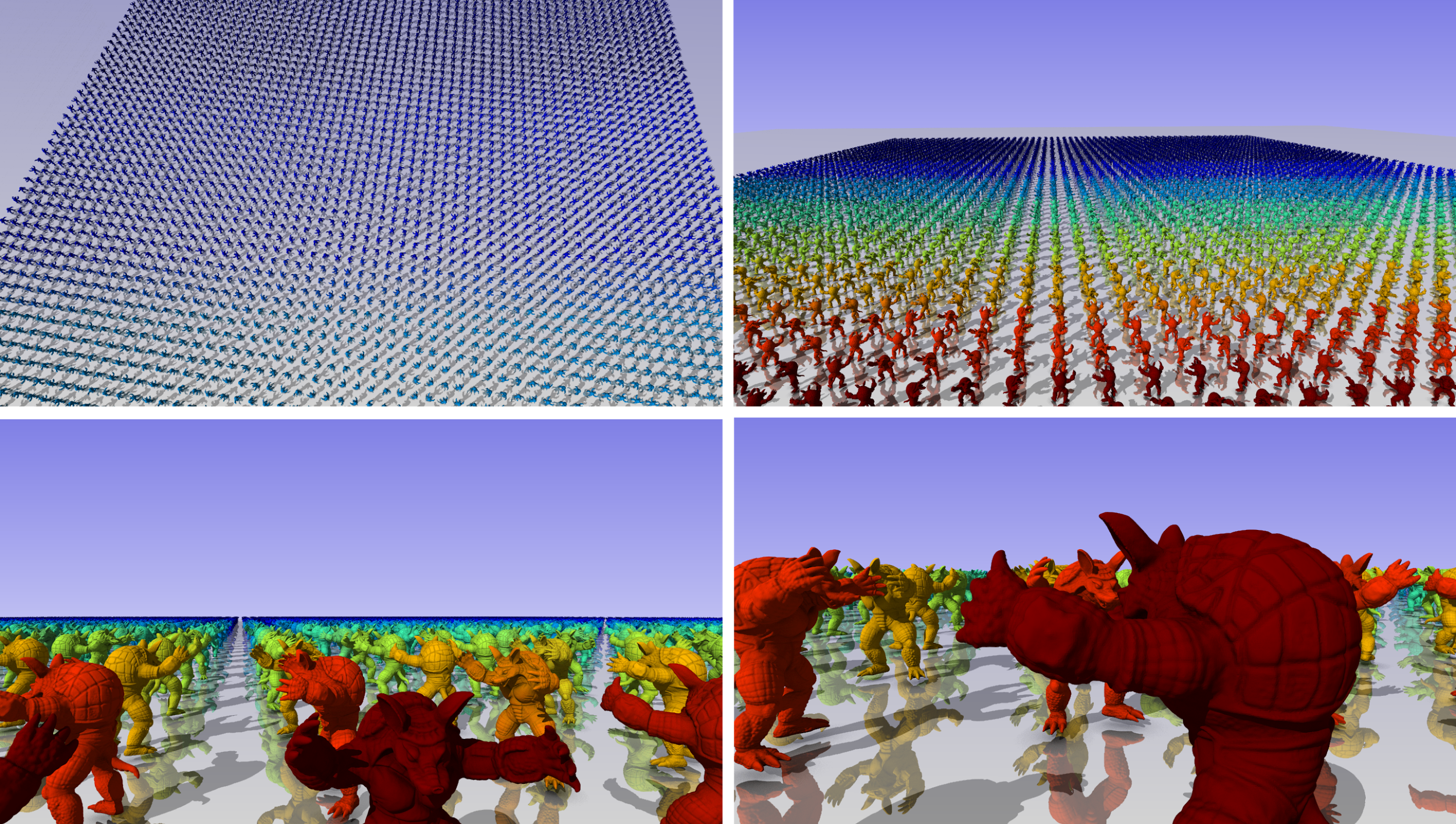
Grid of armadillos seen from different angles and distances. — *Figure 5. The four views used in the benchmark: “top” (upper-left), “high” (upper-right), “low” (lower-left), and “close” (lower-right).*

Figure 5 shows the render timings that we obtained on an NVIDIA GeForce RTX 2080Ti with 64×60 instances and eight LODs. The render time varies depending on the view. Figure 6 also shows that LOD can achieve significant speedups: up to 2.2x for the top view where almost all the objects are rendered at a low LOD.

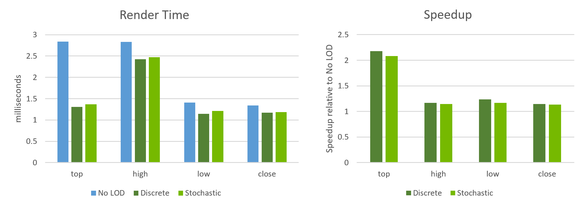
Discrete or stochastic LOD can offer substantial speedups over no LOD, but the amount of speedup varies highly with the specific scenario even in this simple example. — *Figure 6. Render times and speedups for each view.*

As expected, stochastic LOD is slightly slower and has lower speedups than discrete LOD. The other components of frame time, LOD selection time and TLAS build time, are independent of the view. We saw an average LOD selection time of 0.018 ms and TLAS build time of 0.22 ms.

Figure 7 shows the effect of varying the transition interval. This experiment helps to isolate the impact of having neighboring rays use differing ray masks to trace against different objects.

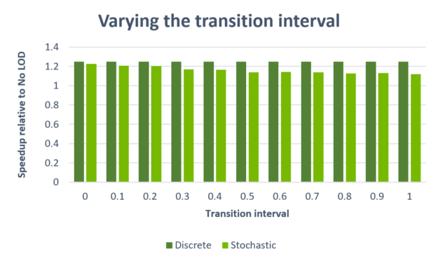
Bar graph showing that increasing the transition interval increases the amount of divergence on average and lowers performance. — *Figure 7. The effect of varying the transition interval for stochastic LOD on the “low” view.*

As the transition interval increases, the amount of divergence between rays increases as well, which negatively affects performance. At a maximum of about 10%, however, this cost is limited. When the transition interval is 0, the rendered result is equivalent to discrete LOD. The only difference then is that you still have two instances per object in the TLAS instead of one. This accounts for only a 1.6% increase in render time.

Conclusion

With this post and the accompanying sample code, we showed a straightforward, discrete LOD mechanism that is in use in various shipping games. We showed that, depending on the situation, the speedups delivered by this mechanism can be significant. We also demonstrated one possible way to implement a fully hardware-accelerated, stochastic LOD approach in DXR that significantly reduces the popping artifacts of discrete LOD with only a small impact on performance.

We encourage you to download the source code and models for the sample here and play with it. Happy experimenting!