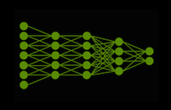
Deep Neural Networks (DNNs) have lead to breakthroughs in a number of areas, including image processing and understanding, language modeling, language translation, speech processing, game playing, and many others. DNN complexity has been increasing to achieve these results, which in turn has increased the computational resources required to train these networks. Mixed-precision training lowers the required resources by using lower-precision arithmetic, which has the following benefits.
- Decrease the required amount of memory. Half-precision floating point format (FP16) uses 16 bits, compared to 32 bits for single precision (FP32). Lowering the required memory enables training of larger models or training with larger minibatches.
- Shorten the training or inference time. Execution time can be sensitive to memory or arithmetic bandwidth. Half-precision halves the number of bytes accessed, thus reducing the time spent in memory-limited layers. NVIDIA GPUs offer up to 8x more half precision arithmetic throughput when compared to single-precision, thus speeding up math-limited layers.
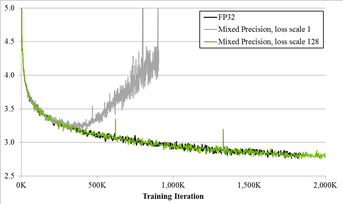
Since DNN training has traditionally relied on IEEE single-precision format, the focus of this this post is on training with half precision while maintaining the network accuracy achieved with single precision (as Figure 1 shows). This technique is called mixed-precision training since it uses both single- and half-precision representations.
Techniques for Successful Training with Mixed Precision
Half-precision floating point format consists of 1 sign bit, 5 bits of exponent, and 10 fractional bits. Supported exponent values fall into the [-24, 15] range, which means the format supports non-zero value magnitudes in the [2-24, 65,504] range. Since this is narrower than the [2-149, ~3.4×1038] range supported by single-precision format, training some networks requires extra consideration. This section describes three techniques for successful training of DNNs with half precision: accumulation of FP16 products into FP32; loss scaling; and an FP32 master copy of weights. With these techniques NVIDIA and Baidu Research were able to match single-precision result accuracy for all networks that were trained (Mixed-Precision Training). Note that not all networks require training with all of these techniques.
For detailed directions on how to apply these techniques in various frameworks, including usable code samples, please see the Training with Mixed Precision User Guide.
Accumulation into FP32
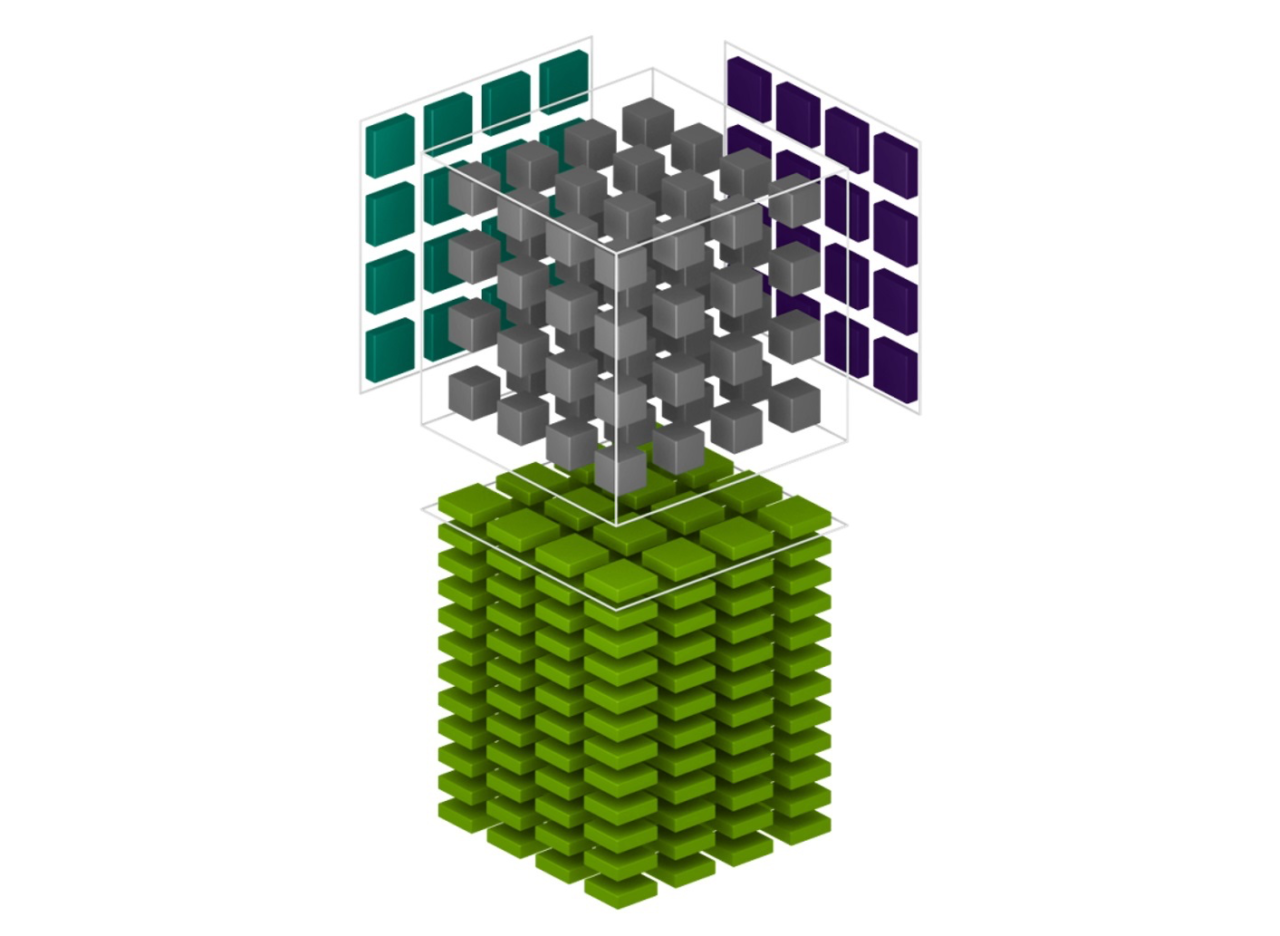
The NVIDIA Volta GPU architecture introduces Tensor Core instructions, which multiply half precision matrices, accumulating the result into either single- or half-precision output. We found that accumulation into single precision is critical to achieving good training results. Accumulated values are converted to half precision before writing to memory. The cuDNN and CUBLAS libraries provide a variety of functions that rely on Tensor Cores for arithmetic.
Loss Scaling
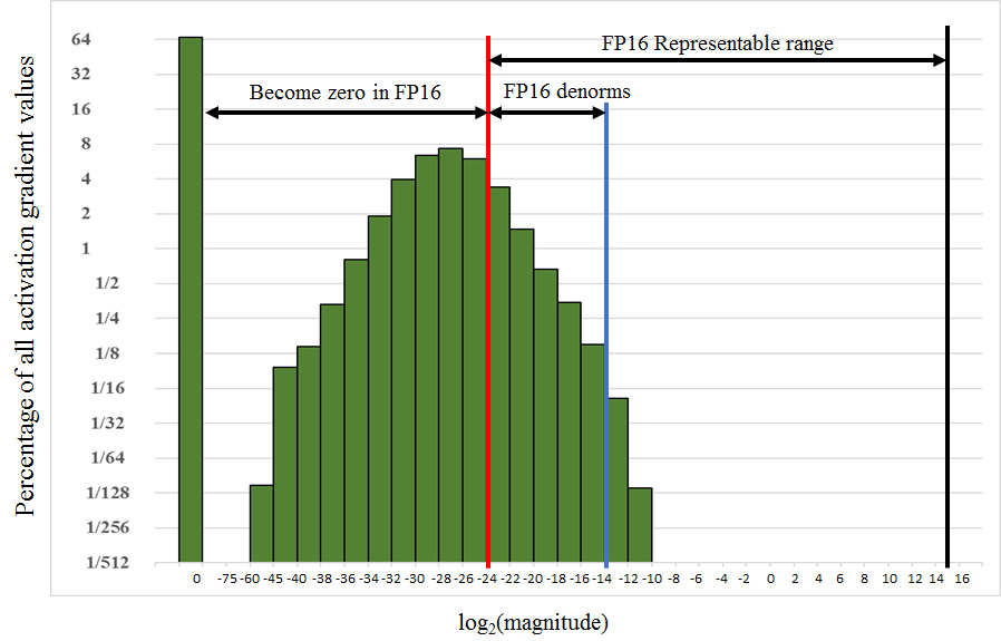
There are four types of tensors encountered when training DNNs: activations, activation gradients, weights, and weight gradients. In our experience activations, weights, and weight gradients fall within the range of value magnitudes representable in half precision. However, for some networks small-magnitude activation gradients fall below half-precision range. As an example, consider the histogram of activation gradients encountered when training the Multibox SSD detection network in Figure 2, which shows the percentage of values on a log2 scale. Values smaller than 2-24 become zeros in half-precision format.
Note that most of the half-precision range is not used by activation gradients, which tend to be small values with magnitudes below 1. Thus, we can “shift” the activation gradients into FP16-representable range by multiplying them by a scale factor S. In the case of the SSD network it was sufficient to multiply the gradients by 8. This suggests that activation gradient values with magnitudes below 2-27 were not relevant to training of this network, whereas it was important to preserve values in the [2-27, 2-24) range.
A very efficient way to ensure that gradients fall into the range representable by half precision is to multiply the training loss with the scale factor. This adds just a single multiplication and by the chain rule it ensures that all the gradients are scaled up (or shifted up) at no additional cost. Loss scaling ensures that relevant gradient values lost to zeros are recovered. Weight gradients need to be scaled down by the same factor S before the weight update. The scale-down operation could be fused with the weight update itself (resulting in no extra memory accesses) or carried out separately. For more details see the Training with Mixed Precision User Guide and Mixed-Precision Training paper.
FP32 Master Copy of Weights
Each iteration of DNN training updates the network weights by adding corresponding weight gradients. Weight gradient magnitudes are often significantly smaller than corresponding weights, especially after multiplication with the learning rate (or an adaptively computed factor for optimizers like Adam or Adagrad). This magnitude difference can result in no update taking place if one of the addends is too small to make a difference in half-precision representation (for example, due to a large exponent difference the smaller addend becomes zero after being shifted to align the binary point).
A simple remedy for the networks that lose updates in this fashion is to maintain and update a master copy of weights in single precision. In each iteration a half-precision copy of the master weights is made and used in both the forward- and back-propagation, reaping the performance benefits. During weight update the computed weight gradients are converted to single-precision and used to update the master copy and the process is repeated in the next iteration. Thus, we’re mixing half-precision storage with single-precision storage only where it’s needed.
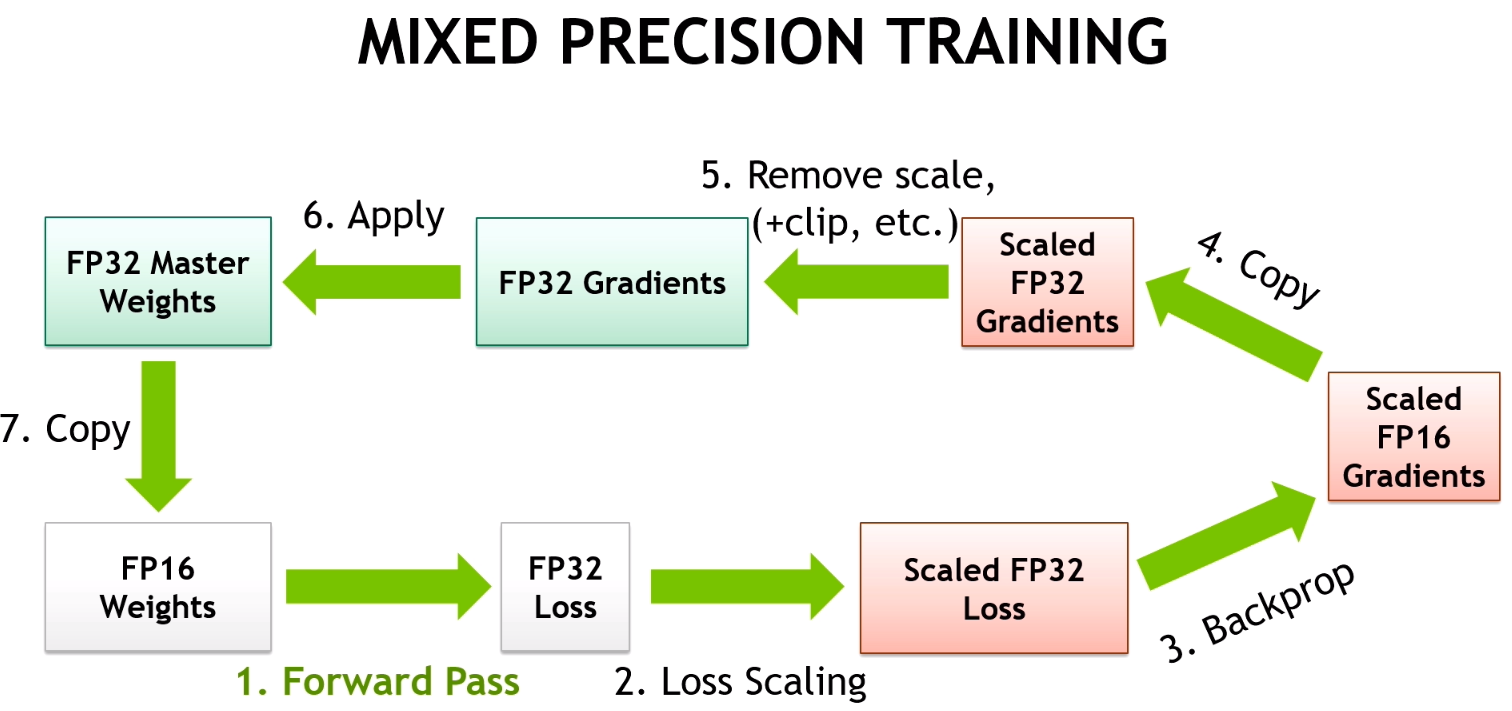
Mixed-Precision Training Iteration
The three techniques introduced above can be combined into the following sequence of steps for each training iteration. Additions to the traditional iteration procedure are in bold.
- Make an FP16 copy of the weights
- Forward propagate using FP16 weights and activations
- Multiply the resulting loss by the scale factor S
- Backward propagate using FP16 weights, activations, and their gradients
- Multiply the weight gradients by 1/S
- Optionally process the weight gradients (gradient clipping, weight decay, etc.)
- Update the master copy of weights in FP32
Examples for how to add the mixed-precision training steps to the scripts of various DNN training frameworks can be found in the Training with Mixed Precision User Guide.
Results
We used the above three mixed-precision training techniques on a variety of convolutional, recurrent, and generative DNNs. Application tasks included image classification, object detection, image generation, language modeling, speech processing, and language translation. For full experimental details please refer to the Mixed-Precision Training paper. Table 1 shows results for image classification with various DNN models. None of the networks in Table 1 needed loss scaling to match single-precision result accuracy. Table 2 shows the mean average precision for object detection networks. Multibox SSD training required loss scaling, and a scale factor of 8 was sufficient to match single-precision training. Without this scaling factor too many activation gradient values are lost to zero and the network fails to train. Recurrent networks tended to require loss scaling and, in many cases, a single-precision master copy of weights. For example, the bigLSTM English language modeling network required a scale factor of 128, without which training eventually diverged as shown in Figure 1. Please refer to the Mixed-Precision Training paper for more networks and training details.
| DNN Model | FP32 | Mixed Precision |
|---|---|---|
| AlexNet | 56.77% | 56.93% |
| VGG-D | 65.40% | 65.43% |
| GoogLeNet | 68.33% | 68.43% |
| Inception v1 | 70.03% | 70.02% |
| Resnet50 | 73.61% | 73.75% |
| DNN Model | FP32 baseline | Mixed Precision without loss-scaling |
Mixed Precision with loss-scaling |
|---|---|---|---|
| Faster R-CNN | 69.1% | 68.6% | 69.7% |
| Multibox SSD | 76.9% | Does not train | 77.1% |
Conclusions
This post briefly introduced three mixed-precision training techniques, useful when training DNNs with half precision. Empirical results with these techniques suggest that while half-precision range is narrower than that of single precision, it is sufficient for training state-of-the-art DNNs for various application tasks as results match those of purely single-precision training. Please have a look at the Mixed-Precision Training paper for a more detailed description of mixed precision training and results for various networks. Refer to the Training with Mixed Precision User Guide for code samples you can use in your own training scripts for various DNN training frameworks.
References
P. Micikevicius, S. Narang, J. Alben, G. Diamos, E. Eelsen, B. Ginsburg, M. Houston, O. Kuchaiev, G. Venkatesh, H. Wu. Mixed Precision Training, 2017. https://arxiv.org/abs/1710.03740
Training with Mixed-Precision User Guide, 2017. http://docs.nvidia.com/deeplearning/sdk/mixed-precision-training/index.html.
B. Ginsburg, S. Nikolaev, P. Micikevicius. Training with Mixed Precision, GPU Technology Conference, 2017. http://on-demand.gputechconf.com/gtc/2017/presentation/s7218-training-with-mixed-precision-boris-ginsburg.pdf