Neural machine translation exists across a wide variety consumer applications, including web sites, road signs, generating subtitles in foreign languages, and more. TensorRT, NVIDIA’s programmable inference accelerator, helps optimize and generate runtime engines for deploying deep learning inference apps to production environments. NVIDIA released TensorRT 4 with new features to accelerate inference of neural machine translation (NMT) applications on GPUs. Google’s Neural Machine Translation (GNMT) model performed inference up to 60x faster using TensorRT on Tesla V100 GPUs compared to CPU-only platforms.
Earlier versions of TensorRT introduced some layers used in recurrent neural networks (RNNs), such as long-short-term memory (LSTM) and gated recurrent units (GRU). The new TensorRT 4 release brings support for new RNN layers such as Batch MatrixMultiply, Constant, Gather, RaggedSoftMax, Reduce, RNNv2, and TopK. These layers allow application developers to accelerate the most compute intensive portions of an NMT model easily with TensorRT. We’ll first look at the architecture of a neural machine translation application, then walk through an example showing how to perform inference for such an application on GPUs. We’ll use the sampleNMT example which ships with TensorRT 4. You can get TensorRT and the sample by downloading the TensorRT container in NVIDIA GPU Cloud and follow along with this tutorial.
Let’s get started by reviewing the architecture of an NMT application and what is new in TensorRT 4.
Neural Machine Translation application overview
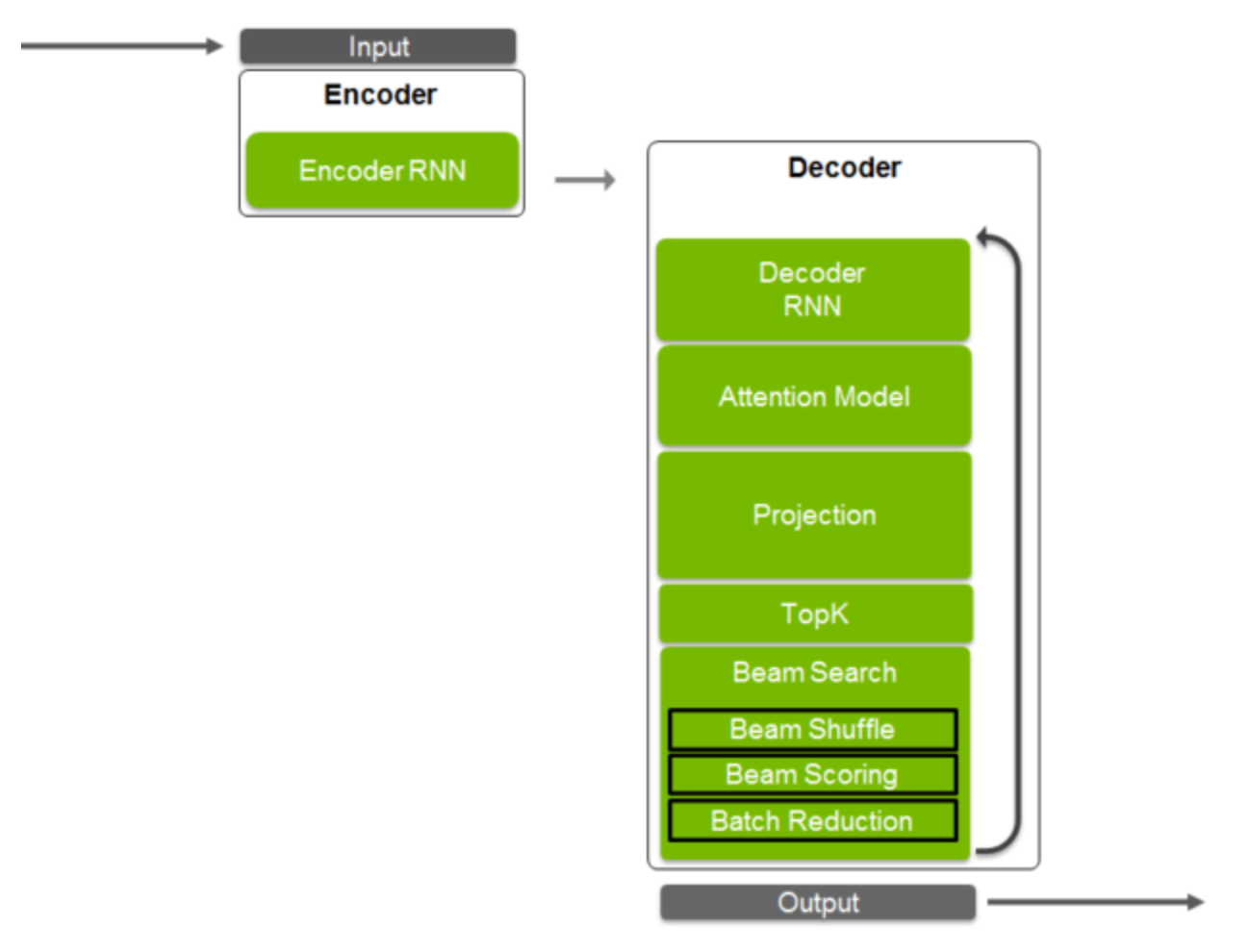
Neural machine translation (NMT) uses deep neural networks to translate text from one language to another language. The translation process starts with tokenizing an input sequence. Tokens can refer to a symbol, character, or word while a sequence can be a word or a sentence. In our example, token refers to a word and sequence refers to a sentence. The sequence is padded with a start and end token; a batch of such sequences are used to train the network to output sequences in another language. NMT models today commonly use sequence-to-sequence models that have an encoder-decoder architecture. See figure 1 for an example architecture of an NMT model. Other variations exist and are used as well.
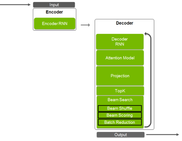
The encoder consists of an RNN that takes the input sequence starting with the start-of-sequence token. Tokens feed into the RNN one at a time till the end-of-sequence token is reached. The goal of the RNN is to capture the “meaning” of the complete sequence in its hidden state. So in the first iteration, the state of the RNN captures only to the start of the sequence token. In the next iteration, the state captures the meaning of first word and the start token. And and so on till the end of sequence is reached. The RNN does much better at capturing the meaning of the most recent tokens fed in to the RNN compared with token encountered at the beginning of the sequence. This becomes a problem for long sequences such as paragraphs. Keep this in mind, we will visit this shortly.
The encoder state is fed to the decoder that uses it to generate a sequence in the target language. The decoder consists of an RNN, attention, projection, topK and beam search. Let’s look at these in more detail. Similar to the encoder, the decoder RNN generates one token at a time starting with the start-of-sequence token using the encoder RNN state as input. As mentioned earlier, this can lose accuracy for longer sequences. Additionally, many languages have similar structure. For example, the first word in an English sequence likely has a strong influence on the first word in the German translation. However, the current architecture does not take advantage of such similarity in structure. One idea is to train the model on the reverse of the input sequence, so the last token that the RNN trains is the beginning of the sequence. When the decoder generates the translated sequence, the first token corresponds to the first word in the sequence and is closest to the beginning of the input sequence, leading to better translations. However, such a method is not generalizable across language pairs, one of the strengths of NMT. The attention model helps address this issue.
Attention uses states from different stages of the input training sequence to help the decoder focus on specific parts of the input sequence. It clips the irrelevant portions of the decoder RNN to the next layer. So far, all the tokens are captured as discrete inputs. The projection layer converts inputs from a discrete space to a continuous space. Conceptually, tokens with similar context get placed close to each other in the continuous feature space. The output of the projection layer consist of probabilities of the likelihood of each token in the vocabulary. This layer creates a large output vocabulary which requires substantial compute capability and memory. The TopK layer selects the top K items with the highest probabilities of likelihood. TopK is a partial sorting algorithm that returns the top K token with highest probability values. For K equal to one, the layer returns the one most likely token in the machine. If K is 3, you will get the top 3 tokens as output from this layer. Now you can either try to predict only a single output sequence from the decoder. Or, you can predict multiple possible output sequences in parallel and finally select the best overall performing sequence. Beam search refers to the technique to process multiple sequences in parallel. The beam width (K1 in our case) is the number of sequences handled simultaneously. Let’s walk through an example when K = 3.
In the first iteration, three tokens are selected as the output of the projection layer. These inputs then feed back to the decoder RNN and passed through the attention and projection layers. For each of the three tokens, the TopK layer selects the top three tokens. This makes total number of tokens being handled by the algorithm 3^2 = 9. The exponential growth in problem size with each iteration quickly becomes a problem. We need to perform a topk reduction across all the beams in order to handle this. This selects the 3 most likely tokens from all the possibilities (see figure 2).

To perform beam search, you need to determine the likelihood of a beam and assign a score (‘beam scoring’) to it. Once the top performing beams are selected, they are then arranged from left to right in decreasing order of probability. In the image, see that beam 5 becomes beam 1, and so on. A batch reduction operation is performed to reduce the batch size that is used to launch work for the next iteration by removing all of the sequences that are finished.
This execution path of the sample above is a cyclic graph that feeds the output of the TopK layer back to the decoder RNN. Subsequent sections will describe how you can build cyclic graphs, similar to what’s used in the architecture shown above with TensorRT. TensorRT 4 introduces new operations and layers used within the decoder such as Constant, Gather, RaggedSoftmax, MatrixMultiply, Shuffle, TopK, and RNNv2. The TensorRT layers section in the documentation provides a good reference. Let’s explore a couple of the new layers.
The RaggedSoftMax layer implements cross-channel SoftMax for an input tensor containing sequences of variable lengths. Using an input set with variable length elements differentiates RaggedSoftMax from the older SoftMax layer. Using variable length computations provides more accurate results and faster computations. A second tensor input specifies the sequence lengths to the layer. RNNv2 offers a new API significantly easier to use than the earlier version, RNNv1. RNNv2 adds to the original by implementing recurrent layers such as RNNs, Gated Recurrent Units (GRUs), and Long Short-Term Memory (LSTM). The older RNN layer has been deprecated in favor of this new version but will continue to work, facilitating backward compatibility.
Let’s run the sample
The sampleNMT sample implements German to English translation and is trained as per the TensorFlow NMT tutorial (https://github.com/tensorflow/nmt). The sample is highly modular and can be used as a starting point for your machine translation application. sampleNMT is located in the tensorrt/samples/sampleNMT directory, which also includes the README.txt file with detailed instructions on how to train and run inference on the sample.
The model was trained on the German to English (De-En) dataset in the WMT database. We need a couple of things in order to run inference:.
- Trained model weights. The De-En weights from the trained model, directly usable by the sample, can be fetched from here and are in the deen/weights folder. The readme.txt provides instructions on how to train the model with TensorFlow, import weights, convert them to binary format usable by the sample and import the weights into a TensorRT model. While this example starts with a model trained in TensorFlow, a similar workflow to bring in weights from any framework of your choice.
- Text and vocabulary data for performing inference. This data for the De-En model, described here, can be fetched using the script wmt16_en_de.sh. See snippet below to import and set up this data. This step might take some time since it prepares 4.5M samples for training as well as inference.
See the code snippet below to learn how to import and set up this data. This step might take some time since it prepares 4.5 million samples for training as well as inference.
# <tensorrt_data_folder> = ‘<path_to_tensorrt>/data’
mkdir -p <tensorrt_data_folder>/nmt/deen; cd <tensorrt_data_folder>/nmt
wget <u><a href="https://raw.githubusercontent.com/tensorflow/nmt/master/nmt/scripts/wmt16_en_de.sh" target="_blank" rel="noopener">https://raw.githubusercontent.com/tensorflow/nmt/master/nmt/scripts/wmt16_en_de.sh</a></u>
chmod 744 wmt16_en_de.sh ; ./wmt16_en_de.sh ; cd 'wmt16_de_en'
cp newstest2015.tok.bpe.32000.de  newstest2015.tok.bpe.32000.en  vocab.bpe.32000.de  vocab.bpe.32000.en <tensorrt_data_folder>/nmt/deen/.
cd <tensorrt_data_folder>/nmt
wget <u><a href="https://developer.download.nvidia.com/compute/machine-learning/tensorrt/models/sampleNMT_weights.tar.gz" target="_blank" rel="noopener">https://developer.download.nvidia.com/compute/machine-learning/tensorrt/models/sampleNMT_weights.tar.gz</a></u>
tar -xzvf sampleNMT_weights.tar.gz
mv ./samples/nmt/deen/weights deen/
Run the command make in the samples/sampleNMT/ directory to build the example. It generates the executable, sample_nmt in the tensorrt/bin directory. Perform inference with command below:
<path_to_tensorrt>/bin/sample_nmt --data_dir=<tensorrt_data_folder>/deen
Let’s look through these options:
--data_dir—Pass the location of the data directory to the sample--data_writer—Example translations can then be found in the translation_output.txt file.--max_inference_samples—Get the BLEU score for the first 100 sentences.
See the full list of available options and their descriptions, use the --help command line option. The sample outputs the following on the command prompt:
data_dir: /workspace/tensorrt/samples/sampleNMT/data/deen
data_writer: text
Component Info:
– Data Reader: Text Reader, vocabulary size = 36548
– Input Embedder: SLP Embedder, num inputs = 36548, num outputs = 512
– Output Embedder: SLP Embedder, num inputs = 36548, num outputs = 512
– Encoder: LSTM Encoder, num layers = 2, num units = 512
– Decoder: LSTM Decoder, num layers = 2, num units = 512
– Alignment: Multiplicative Alignment, source states size = 512, attention keys size = 512
– Context: Ragged softmax + Batch GEMM
– Attention: SLP Attention, num inputs = 1024, num outputs = 512
– Projection: SLP Projection, num inputs = 512, num outputs = 36548
– Likelihood: Softmax Likelihood
– Search Policy: Beam Search Policy, beam = 5
– Data Writer: Text Writer, vocabulary size = 36548
End of Component Info
Note: the sample might generate low BLEU scores in some cases when using trained weights included with the sample. This because because the dictionary implementation during vocabulary generation can vary across python versions and builds. The version you are using might be different from those used to train the model and generate weights. You can resolve this issue by retraining the model to generate new weights.
sampleNMT model architecture
Let’s look at the implementation of the neural machine translation application using TensorRT. The sample implements three TensorRT engines, demonstrating how to orchestrate them for a translation application. The three TensorRT engines in the application are: Encoder, Generator and Beam Shuffle. Figure 3 shows the architecture of the application with layers within each engine, buffers allocated, and portions run on the CPU and CPU. The layers, implemented as components do not directly run computation tasks on the GPU. Instead they add new layers to TensorRT network. This enables TensorRT to apply various optimizations to the execution graph including fusions, in place concatenations, and reduced precision math before execution.
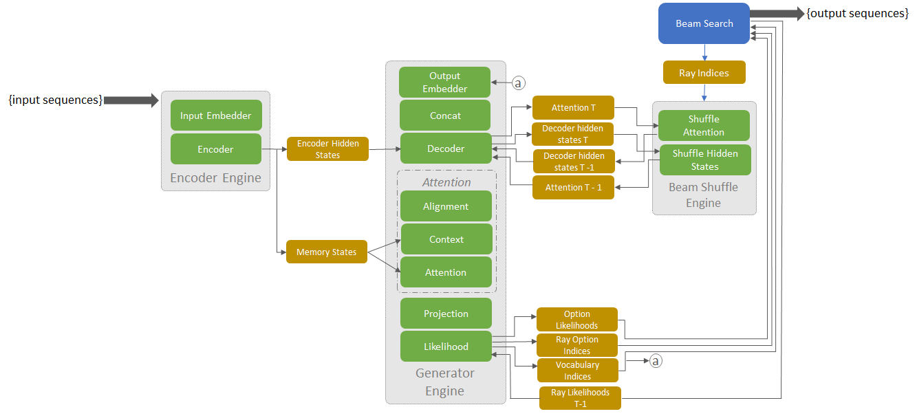
The main function in the sample starts with instantiating layer objects and securing buffers needed for them. After binding the buffers to the layers, the TensorRT engines are created from the layers. In the main execution loop, the encoder engine runs once for each batch of input sequences, generating memory states and hidden states of the encoder. Thes memory and hidden states are used to initialize the Attention mechanism and Decoder correspondingly. Then the app runs Generator and Beam Shuffle engines in the loop until translations for all sequences in the batch are generated. In the sample, both the Top-K operations, intra-beam and reduction across beams, are performed in the likelihood block. One thing to note is that TensorRT supports directed acyclic graphs and this sample demonstrates how to build cyclic graphs formed in auto-regressive models.
Extending the sample for your application
You can extend the sample as needed for your own translation application due to its modular nature. The TensorRT engines generated in the sample use components that abstract the process of setting up network definitions. The sample defines multiple abstract classes, such as Encoder, Embedder, Attention, Decoder, and so on. Each component has at least one pure virtual method to add its definition to the TensorRT network definition. For example, see the method for Embedder component below:
virtual void addToModel(
   nvinfer1::INetworkDefinition* network,
   nvinfer1::ITensor* input,
   nvinfer1::ITensor** output)
= 0;
This method takes a TensorRT tensor containing tokens (integer IDs) of the input sequences. The output should be a tensor, which the function needs to instantiate, and should contain the embedded input. The sample inherits all those components and implements popular cases. For example, it defines SLPEmbedder class, which acts as a lookup table:
void SLPEmbedder::addToModel(
   nvinfer1::INetworkDefinition* network,
   nvinfer1::ITensor* input,
   nvinfer1::ITensor** output)
{
   nvinfer1::Dims weightDims{2, {mNumInputs, mNumOutputs}, {nvinfer1::DimensionType::kCHANNEL, nvinfer1::DimensionType::kCHANNEL}};
   auto constLayer = network->addConstant(weightDims, mKernelWeights);
   assert(constLayer != nullptr);
   constLayer->setName("Embedding matrix");
   auto weights = constLayer->getOutput(0);
   assert(weights != nullptr);

   auto gatherLayer = network->addGather(*weights, *input, 0);
   assert(gatherLayer != nullptr);
   gatherLayer->setName("Gather in embedding");
   *output = gatherLayer->getOutput(0);
   assert(*output != nullptr);
}
You’ll need to implement it the way SLPEmbedder is implemented above to make the sample work with your own specific Embedder, and have nmtSample::getInputEmbedder function return your own implementation:
nmtSample::Embedder::ptr getInputEmbedder()
{
   auto weights = std::make_shared<nmtSample::ComponentWeights>();
   std::ifstream input(locateNMTFile(gEncEmbedFileName));
   assert(input.good());
   input >> *weights;
   return std::make_shared<nmtSample::SLPEmbedder>(weights);
}
And that’s it! The same technique can be used to modify the sample to work with your specific implementation of other components in the application.
Input data reader and output data writer also comprise components. In the scope of the sample, we implemented TextReader which loads textual data from an input stream (for example, from a file). We also added 3 different implementations for the DataWriter: TextWriter, BLEUScoreWriter, and BenchmarkWriter. They write generated translations to text file, compare them to the reference translations and generate a BLEU1 score, respectively, and measure the performance with respect to a benchmark.
TextWriter generates textual translation output, which can be compared with the output from Tensorflow model, provided the weights, test data and vocabularies are identical. The BLEUScoreWriter implementation is based on the one used in the Tensorflow NMT tutorial. BenchmarkWriter disables both BLEU score calculation and generating any output.
You can develop your own implementation of reader and writer components using the process described for the embedder component above. For example, you could implement a service which accepts requests for online translation, batches them together for higher computational efficiency, and dispatches output sequences back to requestors.
Implementing reader and writer are quite straightforward, for example for the DataReader you will need to implement read function:
/**
* \brief reads the batch of samples/sequences
*
* \return the actual number of samples read
*/
virtual int read(
   int samplesToRead,
   int maxInputSequenceLength,
   int* hInputData,
   int* hActualInputSequenceLengths)
= 0;
Profiling and optimizing performance
Let’s look at an example of performance analysis using the data-writer-benchmark component. The benchmark component uses TensorRT’s profiling functionality to explore how much time each component takes to execute. Switch the component on with –profile command line option and use it to analyze the performance of individual components and identify bottlenecks, like so:
./sample_nmt --data_writer=benchmark --profile
========== Host profile ==========
TensorRT layer name                                                   Runtime, %  Invocations  Runtime, ms
Beam Search                                                           79.6%       1022         25.65
Data Read                                                             16.3%         18          5.24
Data Write                                                             0.2%         17          0.05
Intra-batch Sort                                                       3.0%         17          0.98
Read Result                                                            0.9%         17          0.30
========== Host total runtime = 32.2188 ms ==========
========== Encoder profile ==========
TensorRT layer name                                                    Runtime, %  Invocations  Runtime, ms
Attention Keys MM in multiplicative attention                          9.4%        17           13.73
Embedding matrix                                                       0.0%        17            0.04
Gather in embedding                                                    4.4%        17            6.48
LSTM encoder                                                          84.8%        17          123.95
Matrix in multiplicative attention                                     0.0%        17            0.05
Replicate encoder states for decoder initialization 0                  0.4%        17            0.62
Replicate encoder states for decoder initialization 1                  0.4%        17            0.56
Replicate input sequence lengths for decoder                           0.3%        17            0.44
Reshape encoder states for decoder initialization 0                    0.1%        17            0.15
Reshape encoder states for decoder initialization 1                    0.1%        17            0.15
========== Encoder total runtime = 146.169 ms ==========
========== Decoder profile ==========
TensorRT layer name                                                    Runtime, %  Invocations  Runtime, ms
(Unnamed ITensor* 10) copy                                             0.4%        1022         8.98
(Unnamed ITensor* 16) copy                                             0.4%        1022        10.68
(Unnamed ITensor* 19) copy                                             0.4%        1022         9.69
Attention Matrix                                                       0.1%        1022         3.01
Attention Matrix Multiply                                              2.7%        1022        70.46
Context Matrix Multiply                                                2.7%        1022        70.21
Context Ragged Softmax                                                 0.5%        1022        11.84
EltWise multiplication in likelihood calculation                       0.3%        1022         8.26
Embedding matrix                                                       0.1%        1022         3.33
Gather in embedding                                                    1.0%        1022        25.47
LSTM decoder                                                          19.1%        1022       488.98
Projection Matrix Multiply                                            40.6%        1022      1040.08
Projection matrix                                                      0.1%        1022         3.05
Raw Alignment Scores MM (Queries x Keys) in multiplicative attention   4.8%        1022       122.99
Replicate beam likelihoods                                             0.9%        1022        24.35
Reshape combined likelihoods                                           0.3%        1022         6.77
Reshape input for LSTM decoder                                         0.3%        1022         8.68
Reshape output from LSTM decoder                                       0.4%        1022        10.20
Reshape vocabulary indices                                             0.2%        1022         6.38
Shuffle vocabulary indices                                             0.7%        1022        17.83
Softmax in likelihood calculation                                     15.5%        1022       398.48
TopK 1st in likelihood calculation                                     7.4%        1022       188.83
TopK 2nd in likelihood calculation                                     0.7%        1022        17.30
input_attention copy                                                   0.3%        1022         8.64
========== Decoder total runtime = 2564.47 ms ==========
========== Beam shuffle profile ==========
TensorRT layer name                                                   Runtime, %  Invocations  Runtime, ms
Shuffle attention                                                     23.1%       1005         21.28
Shuffle decoder states 0                                              42.5%       1005         39.15
Shuffle decoder states 1                                              34.3%       1005         31.59
========== Beam shuffle total runtime = 92.0182 ms ==========
Notice a few interesting things:
- The host takes only about 1% of the total runtime. The remaining 99% is TensorRT running on the GPU. This occurs for two main reasons. First, the CPU runs only the essentials of the beam search; the beam shuffle runs entirely on the GPU. Second, the sample reads input data for the next batch simultaneously with running the current one to utilize GPU more efficiently and increase inference throughput.
- “Intra-batch Sort” takes just 0.03% of total runtime. Longer input sequences tend to produce longer output translations. Sorting input sequences in the descending order of their lengths allows the sample to efficiently reduce batch size as it generates output sequences since shorter input sentences tend to produce shorter output translations. We saw up to 1.7x performance improvement on batch 128 when applying this trick. Of course, the benefit depends on the specific problem.
Why run anything on the host CPU, even if it takes negligible amount of time? Beam search is a recursive process whitch TensorRT can’t currently handle in its entirety on the GPU. Futhermore, we dynamically reduce batch size as sentences in the batch complete, which can be performed most efficiently on the host. This sample performs 170 times faster than CPU-only during inference for batch=1 and over 100 times faster for batch size = 641.
We added reduced precision experimental feature which can be switched on with –fp16 command-line option. This substantially improves performance while producing almost the same translations as with fp32 math.
Conclusion
TensorRT 4 is available for download today from the the TensorRT product page and in the TensorRT container in NVIDIA GPU Cloud. We are quite excited about all the new capabilities coming together in TensorRT 4 for accelerating neural machine translation apps. This is a start and we are excited about extending these capabilities to address wider set of NMT architectures and frameworks in future versions. As a next step, refer to the documentation for more information on the sample used in this blog, listen to the GTC 2018 talk on Optimizing NMT with TensorRT which provides more of a behind-the-scenes view into optimizing the OpenNMT sample. Use the comments section below to tell us how you plan to use the new capabilities in TensorRT 4. If you have issues with TensorRT, check the NVIDIA TensorRT Developer Forum to see if other members of the TensorRT community have a resolution. NVIDIA Registered Developer Program can also file bugs at https://developer.nvidia.com/nvidia-developer-program.
References
NMT Tensorflow tutorial from Google: https://github.com/tensorflow/nmt
More benchmarks for WMT German-English: https://github.com/tensorflow/nmt#wmt-german-english
[Papineni et al., 2002] BLEU: a Method for Automatic Evaluation of Machine Translation. Kishore Papineni, Salim Roukos, Todd Ward, and Wei-Jing Zhu. Proceedings of the 40th Annual Meeting of the Association for Computational Linguistics (ACL), Philadelphia, July 2002, pp. 311-318
TensorRT Product Page: https://developer.nvidia.com/tensorrt#tensorrt-whats-new
TensorRT sample documentation: https://docs.nvidia.com/deeplearning/sdk/tensorrt-developer-guide/index.html#nmt_sample