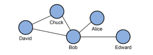
Suppose you want to find the most influential user of Twitter. You would need to know not only how many followers everyone has, but also who those followers are, who the followers of those followers are, and so on. This is a graph problem. Graphs are a mathematical structure that model relationships between entities, whether they’re people, computers, proteins or even abstract concepts.
It turns out that there is already a very popular algorithm for finding the influence of a node in a graph. It’s called PageRank and is the basis of Google’s search algorithm. It has also been used for more important tasks like identifying targets for drugs in disease pathways and identifying ways to destabilize terrorist networks. PageRank is one of many graph algorithms that can be used to solve a myriad of problems.
However, graph analysis presents some unique challenges. Due to the inter-connected nature of the data, individual pieces of the graph cannot be analyzed independently. This is why most graph analysis solutions are designed to perform in-memory analysis. As you can imagine, the Twitter graph and the graph of the Web are each quite large. The cost of in-memory solutions to analyze graphs of this scale, whether they are a single system or a clustered solution, made them cost-prohibitive for some of our customers at Technica.
Another challenge is its reliance on subject matter expertise. As with traditional machine learning, graph analysis requires a data scientist to identify important features of the data and build a solution from several algorithms to solve a larger problem. In the past few years, deep learning has emerged as a data analysis methodology that not only has had great success in numerous fields, but is also able to identify important features in data. In fact, in many cases deep learning solutions have out-performed systems built by subject matter experts with hand-crafted features. We would like to be able to take advantage of this quality by applying deep learning to graph analysis, but this is not straightforward. Deep learning requires regularized input, namely a vector of values, and real world graph data is anything but regular.
Over the past few years, we have been working at Technica IR&D to create a graph analysis solution that can address both of these challenges without sacrificing performance. As aptly demonstrated by the recent release of nvGRAPH, GPUs provide an excellent opportunity for the parallelization of graph analytics tasks. We combine graph algorithms designed specifically for GPUs with an I/O efficient graph partitioning scheme to store graphs on disk. This allows us to use a non-clustered solution without the need for large amounts of RAM. This solution includes the ability to apply deep learning algorithms to graph data in order to simplify analysis. We call our solution FUNL.
Partitioning a Graph
Many graph algorithms are iterative, meaning that they generate a sequence of ever-improving approximate solutions to a problem. At each node a function is applied to values received along incoming edges. The result is then distributed along outgoing edges. In the case of PageRank, the incoming values are summed, a dampening factor is applied and then the result is distributed evenly among outgoing edges.
Since any node can neighbor any other node in the graph, performing these iterative updates can require random access throughout the graph. If the entire graph were held in memory, this would not be as significant a problem. However, we want to store the graph on disk, load a portion of it, perform updates and move on to the next portion, before starting the whole process over again for the next iteration. Naively, this would require random access to the graph on disk.
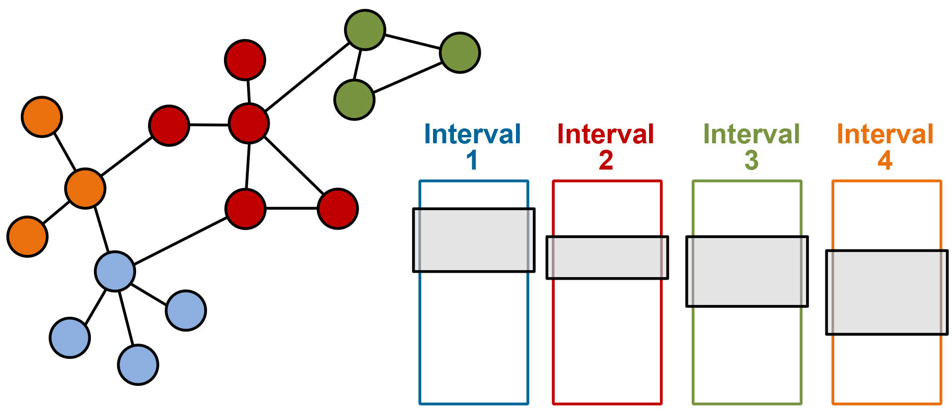
Instead, we use a technique called Parallel Sliding Windows (PSW) to partition the graph so that only a finite number of sequential reads from disk are necessary. PSW is designed for directed graphs, where each edge is directed from a source node to a destination node, but can also be applied to undirected graphs. In this technique, the nodes are broken down into sequential segments called intervals. In Figure 2, each interval of nodes is given its own color. Associated with each interval are all the incoming edges to the nodes of the interval. This collection of edges is called a shard, represented by the colored boxes. Within the shard, the edges are sorted by source and then destination. This means that we can load all in-coming edges to an interval by loading the shard and all out-going edges by loading the corresponding section from all other shards, called windows. Example windows are represented by the gray boxes in each of the shards.
Parallelization of Graph Algorithms
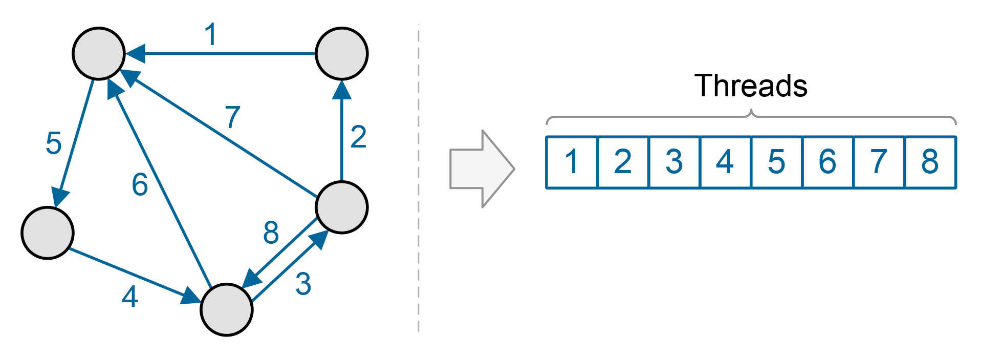
Since graphs consist of many nodes and edges, they present a great opportunity for parallelization. However, which should be our basic work unit, nodes or edges? In general, there are more edges in a graph than nodes. In many real-world graphs there are an order of magnitude more. Also, using edges as our basic work unit provides even load balancing, as the same amount of work must be done for each edge. But this scheme does not provide for data reuse. Each piece of data is operated on once and then discarded, which can prevent us from getting the most performance out of our GPUs.
The alternative is to use the graph nodes as our basic work unit. The advantage is that any function that requires more than one operation per edge, such as a sort of edge labels, allows for greater data reuse. However, this means that we will have an uneven load balance, as some nodes have more neighbors and thus will have more work to do.
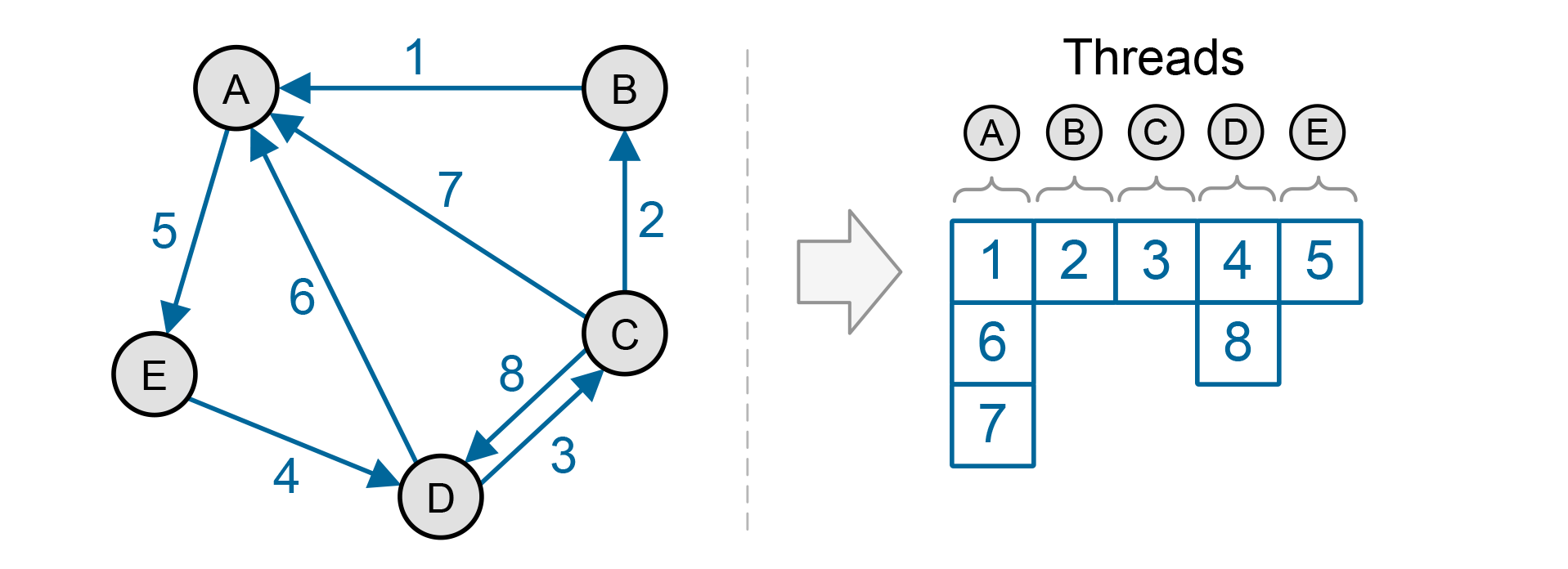
In FUNL, we start by taking the node-centric approach. In order to address the load balancing issue, we divide nodes into two sets, one with nodes that have only a few neighbors and one with nodes that have many. Nodes in the first set are processed using a single thread each, while nodes in the second set are processed using multiple threads.
Performance
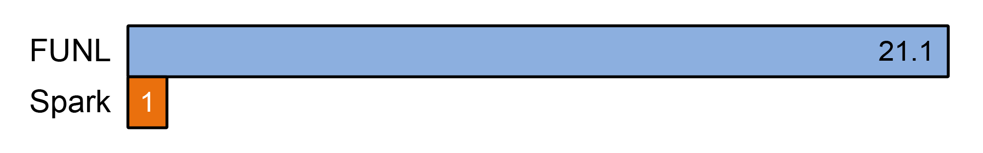
Based on a request from a customer, we compared the performance of FUNL to Apache Spark using the GraphX library. In this case, FUNL ran on a desktop PC with 16GB of RAM, an NVIDIA GeForce GTX Titan GPU and a 180MB/s HDD. Spark ran on an Amazon Web Services cluster of 10 m1.large nodes with moderate network performance. We ran 5 iterations of the PageRank algorithm on a graph with 4.6 million nodes and 77.4 million edges. As you can see in Figure 5, FUNL is approximately 21x faster than Spark. We did not compare against Spark with larger graphs due to the memory requirements of Spark, which would have required an even larger cluster.
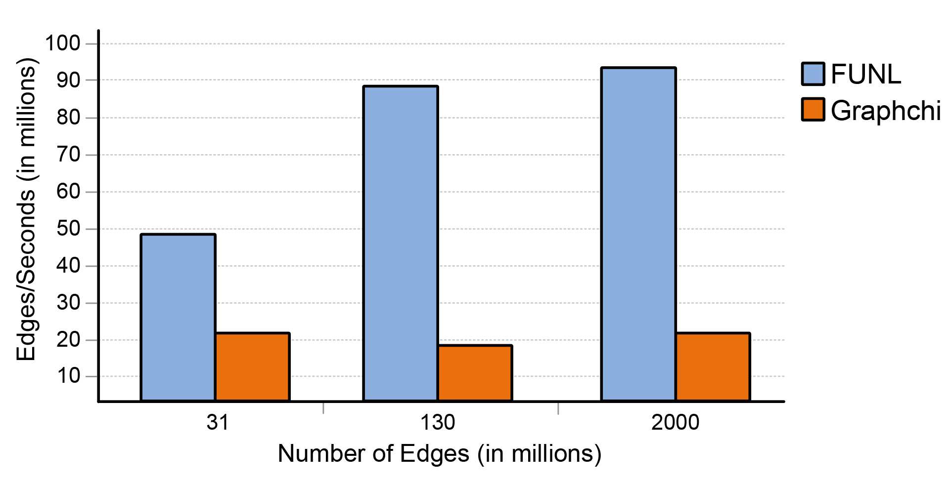
We have also compared FUNL against GraphChi, which is an open source CPU-based graph analysis system that uses the same PSW technique. Both FUNL and GraphChi ran on a system with an Intel Core i7, 64GB RAM and an NVIDIA GeForce GTX Titan Z. In both cases, the graphs were stored on a RAID array. As you can see in Figure 6, utilizing the GPU, FUNL is significantly faster in the 5 iteration PageRank benchmark.
Deep Learning on Graphs with DeepInsight
Consider a more complicated graph analysis task, that of attempting to predict the label of entities in a graph. Suppose we know that some members of a social network are fans of Team A and some are fans of Team B. We may only know this for sure about a very small percentage of the social network and want to make a guess as to which of the other individuals favor which team.
There are a number of ways to approach this task. One is belief propagation, which iteratively computes the conditional probabilities of the possible labels for a node based on the current labels of its neighbors. However, this presupposes that we know something about how the labels relate to one another. Suppose, for example, that neighboring nodes had a tendency to have opposite labels, instead of the same. We would need to know this a priori.
As with other deep learning tasks, we would like to simply provide our training examples to a neural network and then perform some inference. But how would this work with graphs? As mentioned above, graph data is irregular. Any node in a graph can neighbor any other node. We could create a bit vector for each node which indicated whether or not it neighbored each other node, but this is impractical for large graphs that may contain billions of entities.
Our goal then is to generate a representation of each node that encodes the information about its neighborhood in a relatively small and fixed sized vector. There are a number of different ways to accomplish this including extracting locally connected regions of the graph for analysis with convolutional neural networks and using the graph structure itself to build a recurrent neural network. However, we chose to implement an algorithm in FUNL that takes inspiration from natural language processing. The algorithm, called DeepWalk, was developed by Perozzi et al. (2014) at Stonybrook University.
Taking a Walk
Imagine starting from a node in the graph and selecting a neighboring node at random. You move to this node, select a neighbor of the new node at random, and so on. After randomly ‘walking’ some number of steps, you stop. When you are done, you will have created a string of nodes not unlike a sentence. Creating many of these ‘sentences’ will capture much of the information about the graph. In fact, if the graph exhibits a power law distribution, then the node occurrences will as well. As it happens, word usage in natural language exhibits this same exponential behavior.
A common task in natural language analysis is to predict the next word in a sentence. However, since the next node in a walk is random, this prediction has no value. Instead, the algorithm chooses the representation of a node such that maximizes the probability of the preceding and following nodes in the walk. Computing this directly is expensive, so the word2vec is employed to approximate it.
Word2vec uses the hierarchical softmax algorithm, which constructs build a binary tree where each of the leaves represents a node in the original graph. Each of the parent nodes is a binary classifier, so the prediction problem reduces to maximizing the probability of a specific path in the tree given the representation of the neighboring node. This approach reduces the computational complexity of the problem from O(|V|) to O(log|V|). The representation of a node in a random walk is then updated by maximizing the probability of reaching the preceding and following nodes in the binary tree.
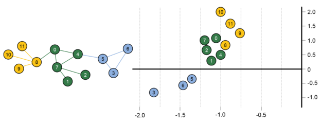
The resulting node representations are quite interesting, as you can see in Figure 7. Nodes that are close together in the 2D representation space have similar neighborhoods in the graph. By identifying tightly clustered nodes in this space, one can detect communities in the original graph. Also, one can draw analogies between the nodes. If two sets of nodes have the same displacement then they will relate to one another the same. For example, in a social network, if a teacher and student have a given displacement, another pair of nodes with the same displacement are likely to also be teacher and student. These node representations can be used to train neural network for label prediction or other graph tasks. One added benefit is that additional features based on non-graph data, such as associated text, can be added to the representations to improve the results of certain tasks.
Perozzi et al. tested this technique for generating node representations against other graph techniques for label prediction, including spectral clustering and modularity based approaches. It outperformed these techniques in many cases, especially for small training data sets.
DeepInsight
This random walk approach to gathering information about the graph lends itself well to parallelization. Since each of the random walks is independent of the others, we implemented the DeepWalk algorithm in FUNL such that each CUDA thread is assigned its own walk. For large graphs, where we are not able to fit the entire graph in GPU memory, we allow the walks to wander until they reach the boundary of a shard. Once all of the walks have gone as far as they can in the current shard, we load the shard that has the most random walks to process. We call our GPU-accelerated implementation DeepInsight.
Results
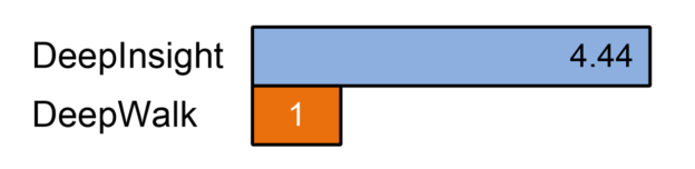
We tested the performance of our implementation against the original DeepWalk implementation. For the random walk portion of the algorithm, our DeepInsight implementation was more than 4 times faster than DeepWalk on a graph with 13M edges. In a preliminary test on a graph with 77M edges, DeepInsight completed the random walks in under 6 minutes, while DeepWalk required well over an hour.
We also tested the efficacy of our implementation on a social network by attempting to distinguish between two types of users. Generating an 8-dimensional representation allowed us to achieve 80% accuracy in predicting the labels. Adding on features generated from the users’ associated improved accuracy to 85%.
Conclusion
With the scale of data growing exponentially, both graph analysis and deep learning are gaining interest. By combining the computational capabilities of GPUs and I/O efficient algorithms, we have demonstrated that large scale graph analysis can be performed on a small budget. While running on a single PC, FUNL has demonstrated significant speedups versus big data systems like Spark and disk-based graph analysis systems like GraphChi.
FUNL’s DeepInsight algorithm adds the ability to analyze large-scale graph data using deep learning techniques. Applying these techniques to graph data opens up many new possibilities and lowers the dependence of graph analysis on subject matter experts. This is really just the beginning, though, as there are many different was to combine these two powerful technologies.
If you’d like to learn more about FUNL, you can visit the Technica innovations page or email us at contactus@technicacorp.com.