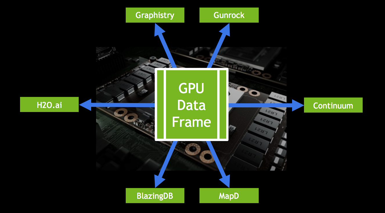
Recently, Continuum Analytics, H2O.ai, and MapD announced the formation of the GPU Open Analytics Initiative (GOAI). GOAI—also joined by BlazingDB, Graphistry and the Gunrock project from the University of California, Davis—aims to create open frameworks that allow developers and data scientists to build applications using standard data formats and APIs on GPUs. Bringing standard analytics data formats to GPUs will allow data analytics to be even more efficient, and to take advantage of the high throughput of GPUs. NVIDIA believes this initiative is a key contributor to the continued growth of GPU computing in accelerated analytics.
Deep learning has propelled GPUs to the forefront of data science. The GPU Technology Conference, held two weeks ago in San Jose, CA, showcased numerous breakthroughs in deep learning, self driving cars, virtual reality, accelerated computing, and more. These advancements are impressive, but I’m even more excited about accelerating the entire data science pipeline with GPUs.
GOAI helps streamline the data pipeline and allows developers to fully utilize the performance of GPUs. Developers can still write their own CUDA C/C++ code to accelerate parts of their workload on GPUs, but this initiative makes GPU-accelerated data science easier. Most data scientists and engineers are familiar with traditional big data tools like Hadoop and Spark and languages like Java, SQL, Scala, Python, and R. In data science, Python, SQL, and R are the leading languages for data manipulation and exploration, with popular packages like Pandas and Data.Table. GOAI will provide access to GPU computing with data science tools commonly used in enterprises applications and Kaggle competitions.
Enabling a GPU Data Science Pipeline
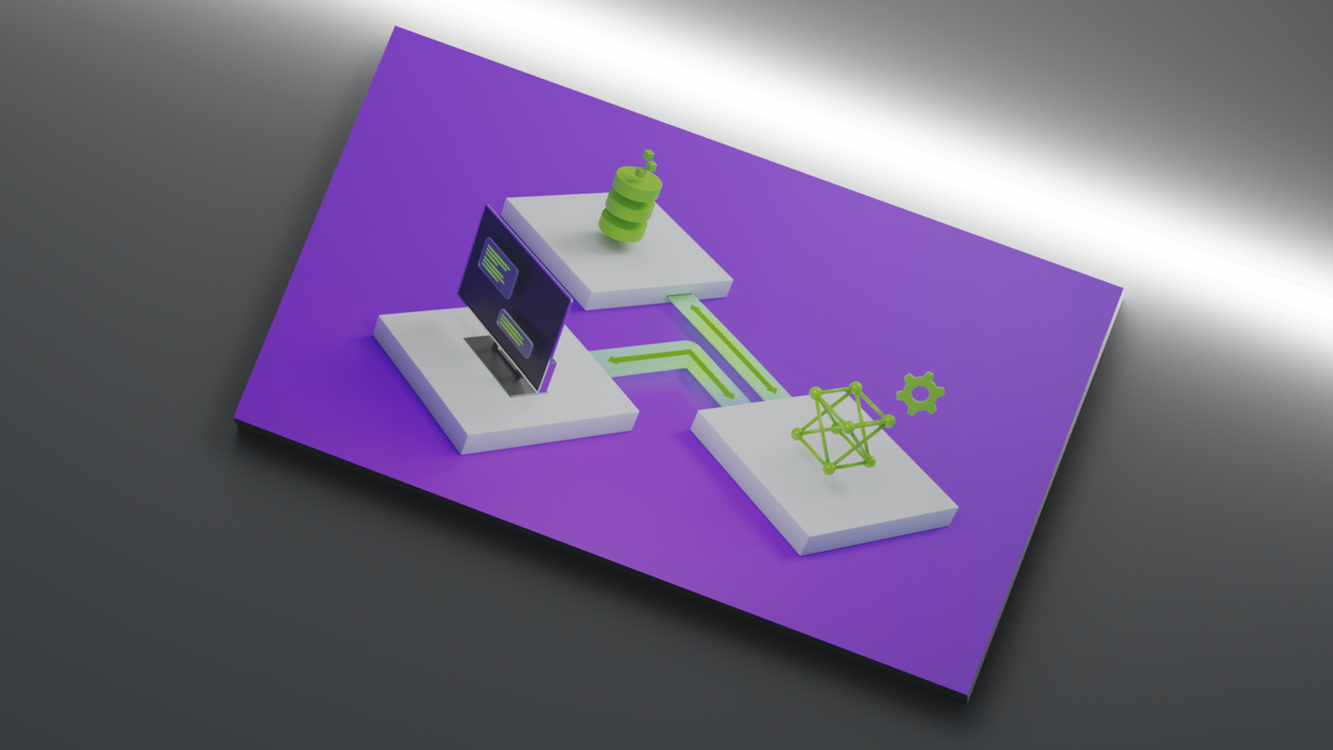
Modern data science workflows typically combine multiple tools, APIs, and technologies. Therefore, shared, standard data structures are essential to building an efficient workflow. Without a shared data structure, workflows have to copy and convert data when going from one tool to another. Today, for two different GPU-accelerated data science applications A and B to talk to each other, A must copy data to the CPU, convert it into another format, and then copy it back to the GPU for B to use it.
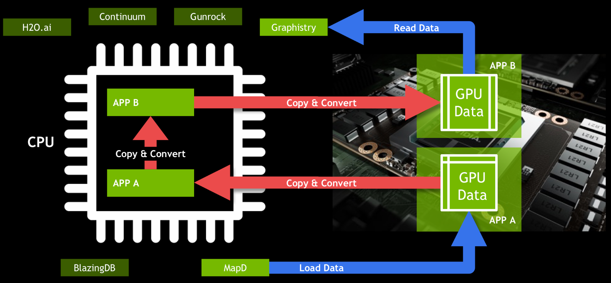
In Figure 1 the data is the same for Applications A and B, but in slightly different formats. Moving data back and forth kills performance, and is inconvenient for end users. GOAI’s first project, the GPU data frame, drastically simplifies the flow of data. The GPU data frame provides an API for efficient data interchange between processes. Once data is loaded into the GPU data frame, any application that uses this common API can access and modify the data without leaving the GPU (Figure 2). This allows users to interact with data using SQL or Python, and then run machine learning algorithms on it, all without transferring the data back to the CPU.

MapD at the Core
In addition to announcing their membership in GOAI, MapD announced that they will open source MapD Core, an extremely fast In-GPU-Memory SQL Database. By opening up their core technology, MapD lays the foundation for the GPU data frame.
To follow along with this post, we suggest downloading a pre-built Docker image as the following example shows. This image combines the GPU data frame, Anaconda, and H2O in a simple demo that predicts income using data from the US Census American Community Survey.
Before downloading the Docker image, make sure you have installed NVIDIA docker. Instructions for installation are available on the NVIDIA Docker GitHub repository. To download, build, and run the demo Docker image, type or paste the following into your terminal.
git clone https://github.com/gpuopenanalytics/demo-docker.git
cd demo-docker
docker build -t conda_cuda_base:latest ./base
docker build -t cudf:latest ./demo
nvidia-docker run -p 8888:8888 -ti cudf:latest
The demo image loads 10,000 rows of census data. Once it’s running it prints a URL in the terminal at which you can access the demo Jupyter notebook. The URL will look something like http://localhost:8888/?token=f6924c055d6019fa8cy0ee5a94108pb95maa44zce449ca1e.
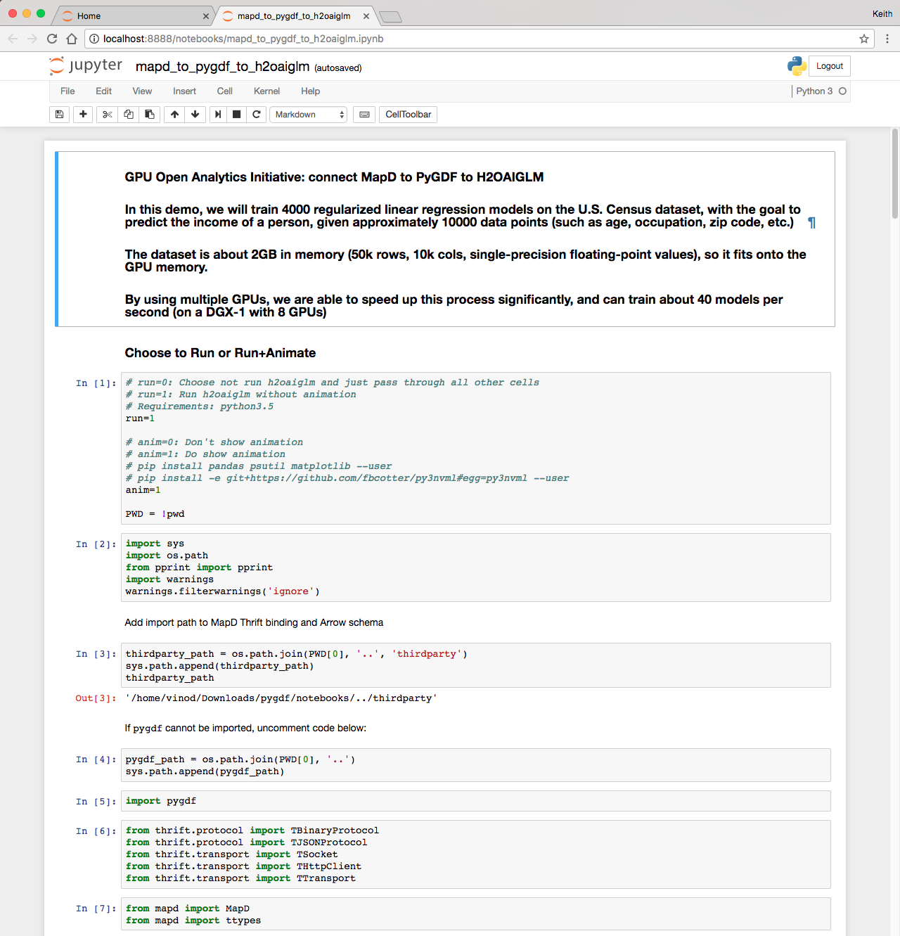
Go to the URL (change localhost to the IP of the machine you’re working off of) and click on the mapd_to_pygdf_to_h2oaiglm.ipynb notebook (Figure 3 shows the notebook). Once the notebook loads, run all the cells (in the menu: Cells -> Run All). Now let’s break down what’s happening in the demo.
The first step creates a table and loads data into MapD via the mapdql command line interface. This is done for you as part of the container creation in a shell script that issues the following commands.
CREATE TABLE ipums_easy (RECTYPE INTEGER, IPUMS_YEAR INTEGER, …);
COPY ipums_easy FROM '~/pygdf/notebooks/ipums_easy.csv';
If you would like to access mapdql in the demo environment you can launch a terminal in Jupyter from the home screen (New -> Terminal). Once you have a terminal, the MapD install directory is /home/appuser/mapd and the mapdql executable is located at /home/appuser/mapd/bin/mapdql. You can run the following commands to start an interactive mapdql session (the default password is “HyperInteractive”).
cd /home/appuser/mapd
./bin/mapdql -p HyperInteractive
To learn more about mapdql, see the documentation.
The notebook first connects to MapD from Python. MapD has Apache Thrift bindings that allow you to interface and connect from any programming language. The following Python code imports a few dependencies and connects to MapD.
from thrift.protocol import TBinaryProtocol
from thrift.protocol import TJSONProtocol
from thrift.transport import TSocket
from thrift.transport import THttpClient
from thrift.transport import TTransport
from mapd import MapD
from mapd import ttypes

def get_client(host_or_uri, port, http):
  if http:
    transport = THttpClient.THttpClient(host_or_uri)
    protocol = TJSONProtocol.TJSONProtocol(transport)
  else:
    socket = TSocket.TSocket(host_or_uri, port)
    transport = TTransport.TBufferedTransport(socket)
    protocol = TBinaryProtocol.TBinaryProtocol(transport)

  client = MapD.Client(protocol)
  transport.open()
  return client
db_name = 'mapd'
user_name = 'mapd'
passwd = 'HyperInteractive'
hostname = 'localhost'
portno = 9091
client = get_client(hostname, portno, False)
session = client.connect(user_name, passwd, db_name)
print('Connection complete')
Once we have a connection to MapD, we can use Thrift to execute a query and keep the results on the GPU.
query = "SELECT {} FROM ipums_easy WHERE INCEARN > 100 order by SERIAL;".format(columns)
results = client.sql_execute_gpudf(session, query, device_id=0, first_n=-1)
GPU-Accelerated Python from Continuum Analytics
Python is arguably the most used programming language in data science, and most data science platforms have Python APIs. Python allows users to efficiently extract, transform, and load (ETL) data to be used by other processes, as well as to mine for insights from data.
The results variable from the previous example is a Thrift handle to the GPU data frame. Next, we need to interface with CUDA from Python using Numba. Numba is a compiler for Python array and numerical functions that gives you the power to speed up your Python applications with high-performance functions. Numba allows you to parallelize loops on GPU or CPU by marking them with decorators and to use GPU-accelerated libraries directly from Python. We’ll access the data frame using the information in the Thrift handle combined with CUDA IPC (inter-process communication) via Numba.
from numba import cuda
from numba.cuda.cudadrv import drvapi

ipc_handle = drvapi.cu_ipc_mem_handle(*results.df_handle)
ipch = cuda.driver.IpcHandle(None, ipc_handle, size=results.df_size)
ctx = cuda.current_context()
dptr = ipch.open(ctx)
Now that we own a pointer (`dptr`) to the data frame in GPU memory, the next step is to point the Python GPU data frame library to it.
import numpy as np

dtype = np.dtype(np.byte)
darr = cuda.devicearray.DeviceNDArray(shape=dptr.size, strides=dtype.itemsize, dtype=dtype, gpu_data=dptr)

from pygdf.gpuarrow import GpuArrowReader
reader = GpuArrowReader(darr)

from pygdf.dataframe import DataFrame
df = DataFrame(reader.to_dict().items())
df is a Python GPU data frame object that we can use to analyze our data. Let’s test that the data frame df is working with Python, by calculating the mean of the earned income variable on the GPU.
df['INCEARN'].mean()
The output is 32876.621408045976.
Next, let’s classify categorical or numerical columns. The number of unique values for each column is calculated on the GPU by the GPU data frame function unique_k(), and each column is classified as categorical if there are fewer than 1000 unique values, or numerical if there are more than 1000 unique values.
uniques = {}
for k in feature_names:
    try:
        uniquevals = df[k].unique_k(k=1000)
        uniques[k] = uniquevals
    except ValueError:
        # more than 1000 unique values
        num_cols.add(k)
    else:
        # within 1000 unique values
        nunique = len(uniquevals)
        if nunique < 2:
            del df[k]        # drop constant column
        elif 1 < nunique < 1000:
            cat_cols.add(k)  # as cat column
        else:
            num_cols.add(k)  # as num column
Now that we have numerical and categorical variables, we should center to the mean and scale componentwise to unit variance: commonly called standardizing. We do this using .scale() in the following code, but first we drop any variable with standard deviation less than .0001 (or infinite). Standardizing numerical values is recommended when running a Generalized Linear Model (GLM), which we will do later.
for k in (num_cols - response_set):
    df[k] = df[k].fillna(df[k].mean())
    assert df[k].null_count == 0
    std = df[k].std()
    # drop near constant columns
    if not np.isfinite(std) or std < 1e-4:
        del df[k]
        print('drop near constant', k)
    else:
        df[k] = df[k].scale()
Next we need to one-hot encode all categorical variables. For example, a one-hot encoding of an education field that can take on the values {HS, SomeCollege, Bachelors, Masters, Doctorate} creates five columns. Each column represents one of the values as either one or zero. One-hot encoding is necessary for GLM, but some algorithms such as random forests do not need one-hot encoding of categorical variables.
for k in cat_cols:
    cats = uniques[k][1:]  # drop first
    df = df.one_hot_encoding(k, prefix=k, cats=cats)
Fast Regressions with H2O
Now we have a sample of data with the necessary transformations. Now let’s run a Generalized Linear Model (GLM) to predict income. GLMs include linear regression, ANOVA, poisson regressions, logistic regressions, and more. In this context, “generalized” means that the response variables can have non-normal error distributions. For more information on GLM please check out the H20 documentation.
The Docker image installed earlier also includes H2O’s GLM. GLM is a great model because it is highly explainable, easy to fit, and accurate even with small data sizes. In industries where explainability is required for regulatory compliance, GLM is a go-to algorithm.
Before we model the data, we split it 80-20 into training and testing subsets, to avoid overfitting the model. This fraction can be set to any value between 0 and 1, but .8 is a common value.
FRACTION=0.8
validFraction=1.0-FRACTION
n60 = int(len(df) * FRACTION)
train_df = df.loc[:n60]
if FRACTION < 1.0:
    test_df = df.loc[n60:]
After we split the data, we turn the training and testing data frames into matrices.
train_data_mat = train_df.as_gpu_matrix(columns=df.columns[1:])
train_result_mat = train_df.as_gpu_matrix(columns=[df.columns[0]])
 if FRACTION < 1.0:
    test_data_mat = test_df.as_gpu_matrix(columns=df.columns[1:])
    test_result_mat = test_df.as_gpu_matrix(columns=[df.columns[0]])
Finally, we pass the matrices to H2O. The zc_void_p command ensures H2O gets the full 64-bit address of the data in GPU memory. Here, we read the 4 matrices into a, b, c, and d.
a=c_void_p(train_data_mat_ptr.value)
b=c_void_p(train_result_mat_ptr.value)
if FRACTION < 1.0:
    c=c_void_p(test_data_mat_ptr.value)
    d=c_void_p(test_result_mat_ptr.value)
Next, we tell H2OAIGLM to remove the mean income (intercept) in order to fit the residual income for more accuracy, and that the data is already standardized so the GLM does not need to do it again.
intercept = 1
standardize = 0
Then we tell H2OAIGLM how many columns (n) and how many rows (mTrain) of training data are present.
n=train_data_mat.shape[1]
mTrain=train_data_mat.shape[0]
Then we tell H2OAIGLM that there are no weights to be applied to each observation, a feature that can be used in the future.
# Not using weights
e=c_void_p(0)
Next, we make the call to H2OAIGLM, passing the locations of the data and problem setup.
enet.fit(sourceDev, mTrain, n, mValid, intercept, standardize, precision, a, b, c, d, e)
In order to avoid fitting to noise in the data, the elastic net GLM (net) fits using regularization in two forms. The first form, L1 lasso regularization, tries to select the most important features (like age). The second form, L2 ridge regularization, tries to suppress complicated fits in favor of simple generalizable fits. These are controlled by the parameter alpha (0 for only L2 and 1 for only L1). The parameter lambda controls the overall regularization. These parameters each vary over the entire span of possible values (0 to 1 for alpha and lambda_min_ratio to 1 or the maximum possible lambda value); they are sampled at NAlphas locations for alpha and NLambdas locations for lambda.
lambda_min_ratio=1E-9
nFolds=5
nAlphas=8
nLambdas=100
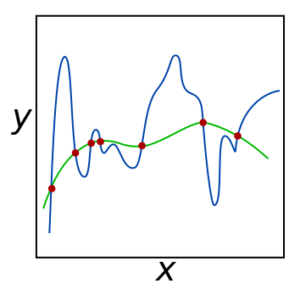
The plot in Figure 4 shows how data points (red) can be fit with a complicated (blue line) or simple (green line) solution. The blue line represents a model that overfits the data and therefore does not generalize well, because it relies too heavily on very specific data values that could be contaminated by noise, vary over time, or differ in each instance for other reasons. The alpha and lambda regularizations help suppress the bad fits.
In order to further regularize the fit to ensure it can generalize well, we also perform cross validation, which removes a portion of training data and uses that portion to test how well the model fits. This is performed nFolds times for each alpha and lambda by removing 1/nFolds of the data for each attempt. This further reduces any erroneous complicated fits that would not generalize well.
Then, we fit the data using the GLM inside H2OAIGLM using these settings (arg). Given 5 folds, 8 alphas, and 100 lambdas, this method will run 4000 models using the maximum number of GPUs on a system (nGPUs = maxNGPUS).
nGPUs=maxNGPUS # choose all GPUs
arg = intercept,standardize, lambda_min_ratio, nFolds, nAlphas, nLambdas, nGPUs
RunH2Oaiglm(arg)
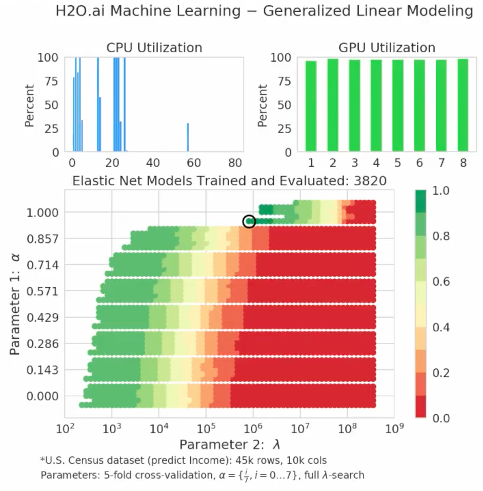
Simultaneously with the fitting process, the notebook shows the resulting grid search results for the accuracy of the model. This shows whether the model actually generalized to data never before used in the model. The top-left panel in Figure 5 shows CPU utilization for each core and the top-right panel shows GPU utilization for each GPU. The bottom panel shows the relative accuracy of the model on the validation set. The validation data was not used to make the model, so can be trusted as an impartial data set to test if the model generalizes well and remains accurate. Red corresponds to no better than using the mean income to predict any income, while green indicates a more accurate model that does much better than just using the mean income to predict the income. The models in green use various features in the data, combined in a linear way, to produce a model that best matches the training data while being expected to generalize well to unseen test data.
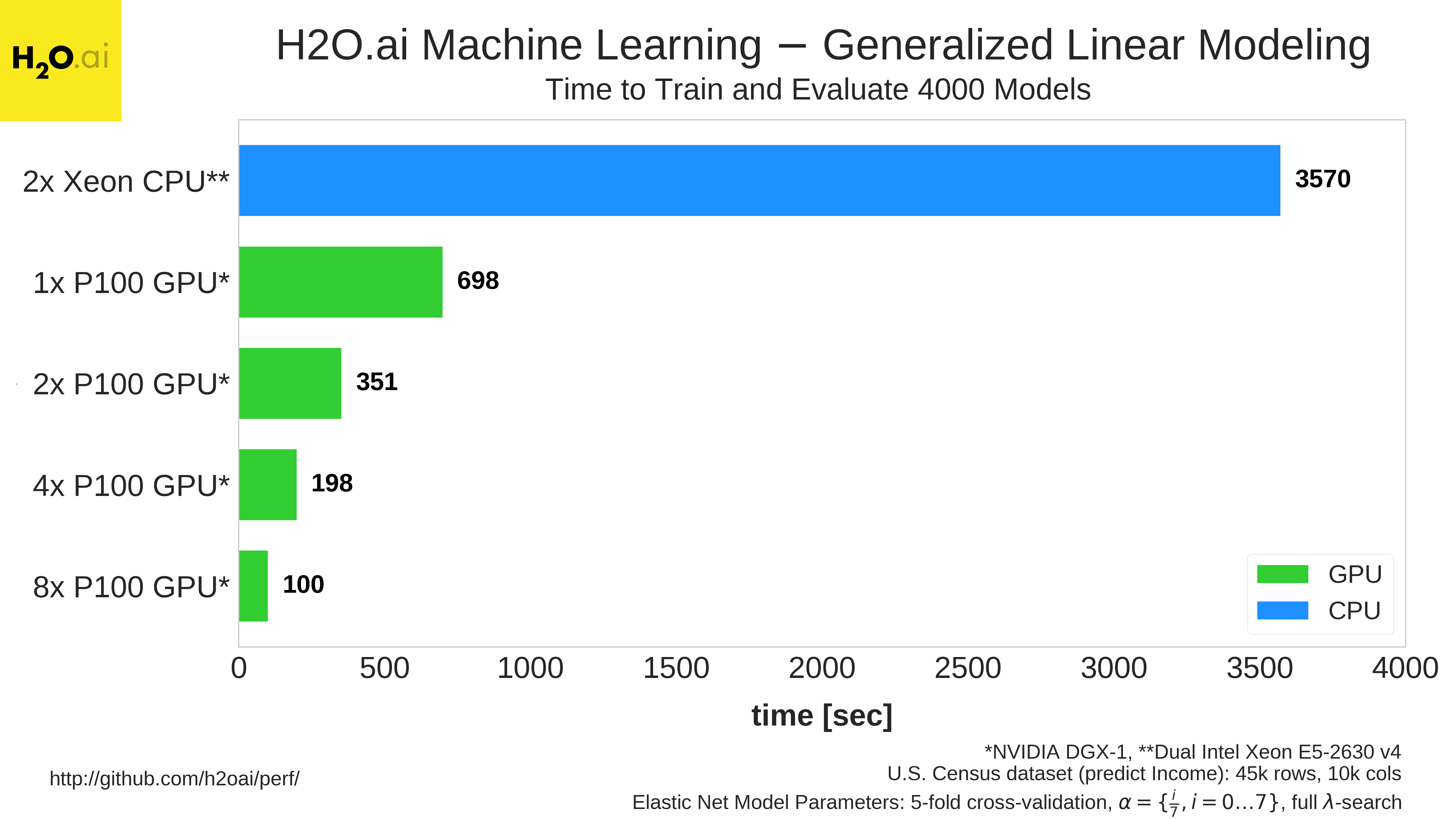
The following video from H2O compares CPU and GPU implementations of GLM.
As the video shows, a DGX-1 with 8x P100s is able to train and evaluate 4000 elastic net models in 100 seconds. On the other hand, by the end of the video, after about 215 seconds have elapsed, the dual Xeon system has only trained and evaluated 209 models. To finish all 4000 models, the dual Xeon system requires 3570 seconds. Figure 6 compares GLM running on multiple GPUs to a dual-Xeon CPU system.
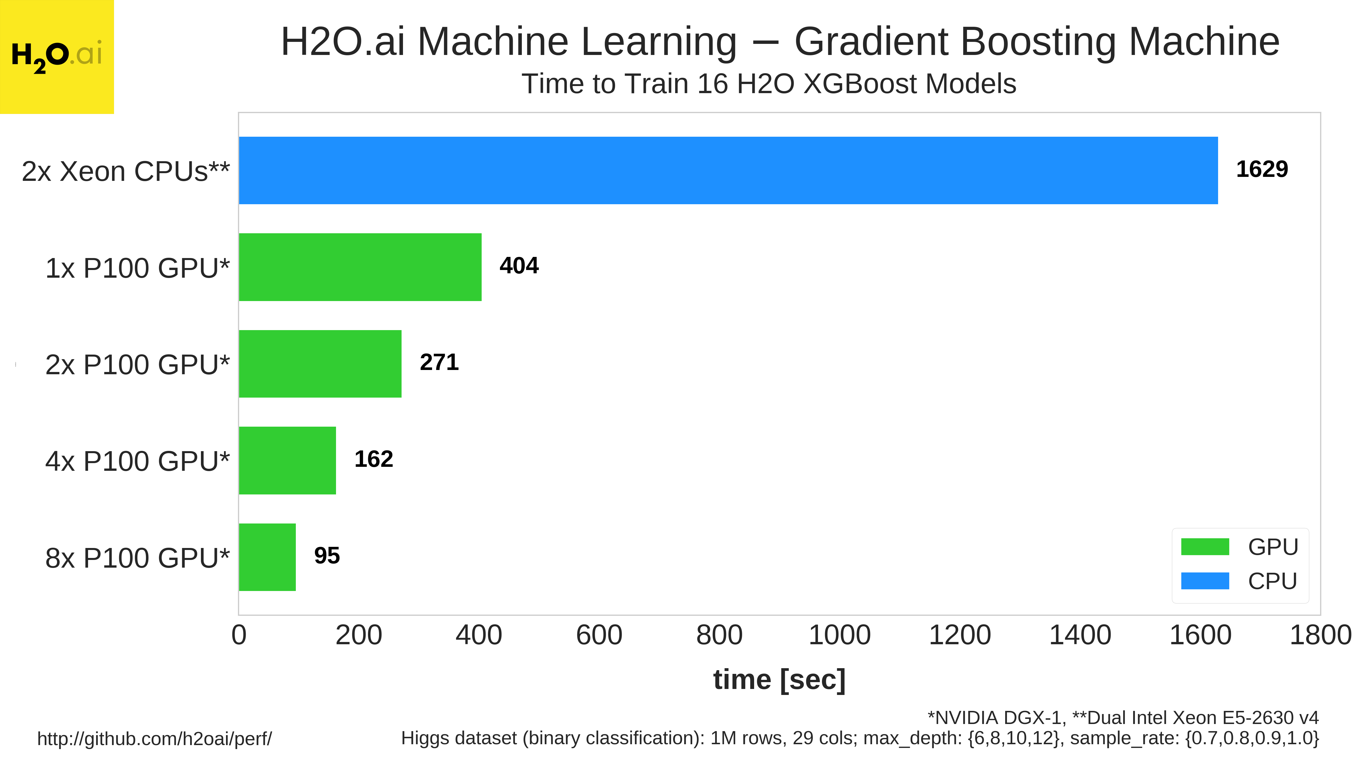
In addition to GLM, H2O Gradient Boosting Machine training also achieves large speedups on NVIDIA GPUs, as Figure 7 shows.
Benchmarking results from H2O are available in their performance benchmarks GitHub repository.
The Beginning of GPU-Accelerated Data Science
GPUs accelerate the most demanding analytical workloads by orders of magnitude. With GOAI, end-to-end GPU workloads are much faster and easier for data scientists to build. In this post we walked through an introductory demo to subset, ETL, and model Census data to predict income.
Currently, the GPU data frame is a single-GPU data structure with support for multi-GPU model-parallel training, where each GPU gets a duplicate of the data and trains an independent model. GOAI plans to add support for multi-GPU distributed data frames and data-parallel training (where GPUs work together to train a model) in the future. In the future, H2O plans to provide additional machine learning models, such as gradient boosting machines (GBM), support vector machines (SVM), k-means clustering, and more, with multi-GPU data-parallel and model-parallel training support. Continuum Analytics will continue to add Python functionality and bring the richness of Anaconda to the GPU. Finally, MapD plans to expand GPU SQL support and data visualization functionality.
We’re excited that organizations are already joining GOAI, including BlazingDB, Graphistry, and Gunrock. Integrating scale-out data warehousing, graph visualization, and graph analytics will give data scientists more tools to analyze even larger and more complex datasets.
We have created a MapD demo to explore this census data. Please visit http://census.mapd.com to visually explore 16 years of the US Census Bureau American Community Survey Public Use Microdata Survey!
Try GOAI GPU Data Frames Today!
The GPU Data Frame, along with its Python API, is the first project of the GPU Open Analytics Initiative aimed at creating common data frameworks that enable application developers and end users to accelerate data science on GPUs. We encourage you to try it out today and join the discussions on the GOAI Google Group and GitHub.
The GPU Data Frame and future projects from GOAI will act as fundamental building blocks for GPU-acceleration in analytics technologies and solutions. GOAI plans to have a production-ready release of the GPU Data Frame by Strata Data Conference New York at the end of September.
Go AI!