This series of blog posts aims to provide an intuitive and gentle introduction to deep learning that does not rely heavily on math or theoretical constructs. The first part in this series provided an overview over the field of deep learning, covering fundamental and core concepts. The third part of the series covers sequence learning topics such as recurrent neural networks and LSTM.
In this second part, we look briefly into the history of deep learning and then proceed to methods of training deep learning architectures quickly and efficiently. The third part focuses on sequence learning, and part four focused on reinforcement learning.
I wrote this series in a glossary style so it can also be used as a reference for deep learning concepts.
History
A Short History of Deep Learning
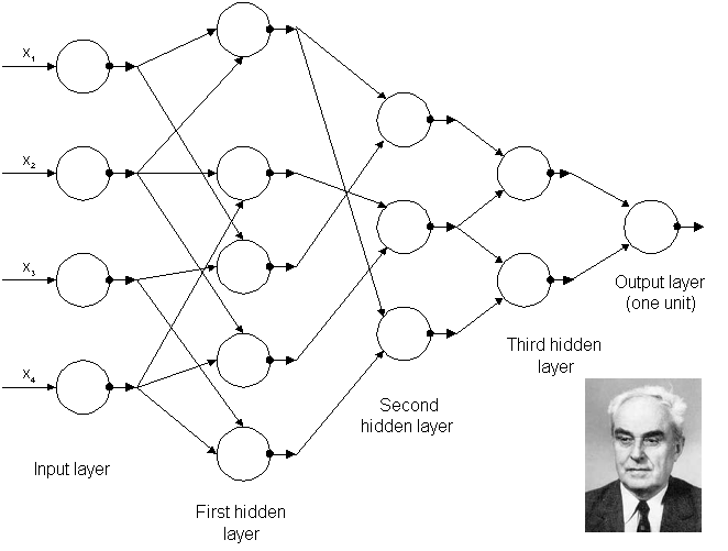
The earliest deep-learning-like algorithms that had multiple layers of non-linear features can be traced back to Ivakhnenko and Lapa in 1965 (Figure 1), who used thin but deep models with polynomial activation functions which they analyzed with statistical methods. In each layer, they selected the best features through statistical methods and forwarded them to the next layer. They did not use backpropagation to train their network end-to-end but used layer-by-layer least squares fitting where previous layers were independently fitted from later layers.
The earliest convolutional networks were used by Fukushima in 1979. Fukushima’s networks had multiple convolutional and pooling layers similar to modern networks, but the network was trained by using a reinforcement scheme where a trail of strong activation in multiple layers was increased over time. Additionally, one would assign important features of each image by hand by increasing the weight on certain connections.
Backpropagation of errors to train deep models was lacking at this point. Backpropagation was derived already in the early 1960s but in an inefficient and incomplete form. The modern form was derived first by Linnainmaa in his 1970 masters thesis that included FORTRAN code for backpropagation but did not mention its application to neural networks. Even at this point, backpropagation was relatively unknown and very few documented applications of backpropagation existed the early 1980s (e.g. Werbos in 1982). Rumelhart, Hinton, and Williams showed in 1985 that backpropagation in neural networks could yield interesting distributed representations. At this time, this was an important result in cognitive psychology where the question was whether human cognition can be thought of as relying on distributed representations (connectionism) or symbolic logic (computationalism).
The first true, practical application of backpropagation came about through the work of LeCun in 1989 at Bell Labs. He used convolutional networks in combination with backpropagation to classify handwritten digits (MNIST) and this system was later used to read large numbers of handwritten checks in the United States. The video above shows Yann LeCun demonstrating digit classification using the “LeNet” network in 1993.
Despite these successes, funding for research into neural networks was scarce. The term artificial intelligence dropped to near pseudoscience status during the AI winter and the field still needed some time to recover. Some important advances were made in this time, for example, the long short-term memory (LSTM) for recurrent neural networks by Hochreiter and Schmidhuber in 1997, but these advances went mostly unnoticed until later as they were overshadowed by the support vector machine developed by Cortes and Vapnik in 1995.
The next big shift occurred just by waiting for computers to get faster, and then later by the introduction of graphics processing units (GPUs). Waiting for faster computers and GPUs alone increased the computational speed by a factor of 1000 over a span of 10 years. In this period, neural networks slowly began to rival support vector machines. Neural networks can be slow when compared to support vector machines, but they reach much better results with the same amount of data. Unlike simpler algorithms, neural networks continue to improve with more training data.
The main hurdle at this point was to train big, deep networks, which suffered from the vanishing gradient problem, where features in early layers could not be learned because no learning signal reached these layers.
The first solution to this problem was layer-by-layer pretraining, where the model is built in a layer-by-layer fashion by using unsupervised learning so that the features in early layers are already initialized or “pretrained” with some suitable features (weights). Pretrained features in early layers only need to be adjusted slightly during supervised learning to achieve good results. The first pretraining approaches where developed for recurrent neural networks by Schmidhuber in 1992, and for feed-forward networks by Hinton and Salakhutdinov in 2006. Another solution for the vanishing gradient problem in recurrent neural networks was long short-term memory in 1997.
As the speed of GPUs increased rapidly, it was soon possible to train deep networks such as convolutional networks without the help of pretraining as demonstrated by Ciresan and colleagues in 2011 and 2012 who won character recognition, traffic sign, and medical imaging competitions with their convolutional network architecture. Krizhevsky, Sutskever, and Hinton used a similar architecture in 2012 that also features rectified linear activation functions and dropout for regularization. They received outstanding results in the ILSVRC-2012 ImageNet competition, which marked the abandonment of feature engineering and the adoption of feature learning in the form of deep learning. Google, Facebook, and Microsoft noticed this trend and made major acquisitions of deep learning startups and research teams between 2012 and 2014. From here, research in deep learning accelerated rapidly.
Additional material: Deep Learning in Neural Networks: An Overview
Perceptron
A perceptron contains only a single linear or nonlinear unit. Geometrically, a perceptron with a nonlinear unit trained with the delta rule can find the nonlinear plane separating data points of two different classes (if the separation plane exists). If no such separation plane exists, the perceptron will often still produce separation planes that provide good classification accuracy. The good performance of the perceptron led to a hype of artificial intelligence. In 1969 however, it was shown that a perceptron may fail to separate seemingly simple patterns such as the points provided by the XOR function. The fall from grace of the perceptron was one of the main reasons for the occurrence of the first AI winter. While neural networks with hidden layers do not suffer from the typical problems of the perceptron, neural networks were still associated with the perceptron and therefore also suffered an image problem during the AI winter.
Despite this, and despite the success of deep learning, perceptrons still find widespread use in the realm of big data, where the simplicity of the perceptron allows for successful application to very large data sets.
AI Winter
Rapid advances in machine learning and other approaches of inference led to a hype of artificial intelligence (similar to the buzz around deep learning today). Researchers made promises that these advances would continue and would lead to strong AI and in turn, AI research received lots of funding.
In the 1970s it became clear that those promises could not be kept, funding was cut dramatically and the field of artificial intelligence dropped to near pseudo-science status. Research became very difficult (little funding; publications almost never made it through peer review), but nevertheless, a few researchers continued further down this path and their research soon lead to the reinvigoration of the field and the creation of the field of deep learning.
This is why excessive deep learning hype is dangerous and researchers typically avoid making predictions about the future: AI researchers want to avoid another AI winter.
AlexNet
AlexNet is a convolutional network architecture named after Alex Krizhevsky, who along with Ilya Sutskever under the supervision of Geoffrey Hinton applied this architecture to the ILSVRC-2012 competition that featured the ImageNet dataset. They improved the convolutional network architecture developed by Ciresan and colleagues, which won multiple international competitions in 2011 and 2012 by using rectified linear units for enhanced speed and dropout for improved generalization. Their results stood in stark contrast to feature engineering methods, which immediately created a great rift between deep learning and feature engineering methods for computer vision. From here it was apparent that deep learning would take over computer vision and that other methods would not be able to catch up. AlexNet heralded the mainstream usage and the hype of deep learning.
ImageNet Classification with Deep Convolutional Neural Networks.
Training Deep Learning Architectures
Training
The process of training a deep learning architecture is similar to how toddlers start to make sense of the world around them. When a toddler encounters a new animal, say a monkey, he or she will not know what it is. But then an adult points with a finger at the monkey and says: “That is a monkey!” The toddler will then be able to associate the image he or she sees with the label “monkey”.
A single image, however, might not be sufficient to label an animal correctly when it is encountered the next time. For example, the toddler might mistake a sloth for a monkey or a monkey for a sloth, or might simply forget the name of a certain animal. For reliable recall and labeling, a toddler needs to see many different monkeys and similar animals and needs to know each time whether or not it is really a monkey—feedback is essential for learning. After some time, if the toddler encounters enough animals paired with their names, the toddler will have learned to distinguish between different animals.
The deep learning process is similar. We present the neural network with images or other data, such as the image of a monkey. The deep neural network predicts a certain outcome, for example, the label of the object in an image (“monkey”). We then supply the network with feedback. For example, if the network predicted that the image showed a monkey with 30% probability and a sloth with 70% probability, then all the outputs in favor of the sloth class made an error! We use this error to adjust the parameters of the neural network using the backpropagation of errors algorithm.
Usually, we randomly initialize the parameters of a deep network so the network initially outputs random predictions. This means for ImageNet, which consists of 1000 classes, we will achieve an average classification accuracy of just 0.1% for any image after initializing the neural network. To improve the performance we need to adjust the parameters so that the classification performance increases over time. But this is inherently difficult: If we adjust one parameter to improve performance on one class, this change might decrease the classification performance for another class. Only if we find parameter changes that work for all classes can we achieve good classification performance.
If you imagine a neural network with only 2 parameters (e.g. -0.37 and 1.14), then you can imagine a mountain landscape, where the height of the landscape represents the classification error and the two directions—north-south (x-axis) and east-west (y-axis)—represent the directions in which we can change the two parameters (negative-positive direction). The task is to find the lowest altitude point in the mountain landscape: we want to find the minimum.
The problem with this is that the entire mountain landscape is unknown to us at the beginning. It is as if the whole mountain range is covered in fog. We only know our current position (the initial random parameters) and our height (the current classification error). How can we find the minimum quickly when we have so little information about the landscape?
Stochastic Gradient Descent
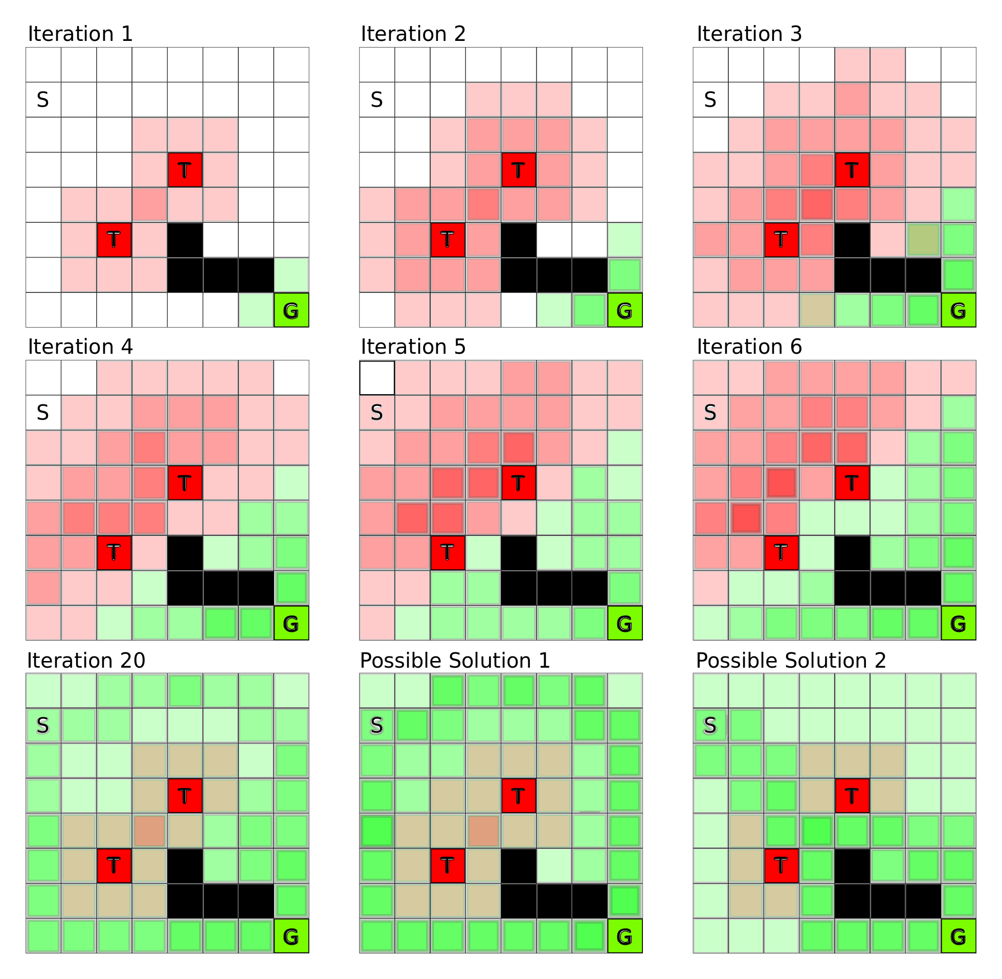
Imagine you stand on top of a mountain with skis strapped to your feet. You want to get down to the valley as quickly as possible, but there is fog and you can only see your immediate surroundings. How can you get down the mountain as quickly as possible? You look around and identify the steepest path down, go down that path for a bit, again look around and find the new steepest path, go down that path, and repeat—this is exactly what gradient descent does.
While gradient descent is equivalent to stopping every 10 meters and measuring the steepness of your surroundings with a measuring tape (you measure your gradient according to the whole data set), stochastic gradient descent is the equivalent of quickly estimating the steepness with a short glance (just a few hundred data points are used to estimate the steepness).
In terms of stochastic gradient descent, we go down the steepest path (the negative gradient or first derivative) on the landscape of the error function to find a local minimum, that is, the point that yields a low error for our task. We do this in tiny steps so that we do not get trapped in half-pipe-like obstacles (if we are too fast, we never get out of these half-pipes and we may even be “catapulted” up the mountain).
While our ski-landscape is 3D, typical error landscapes may have millions of dimensions. In such a space we have many valleys so it is easy to find a good solution, but we also have many saddle points, which makes matters very difficult.
Saddle points are points at which the surroundings are almost entirely flat, yet which may have dramatic descents at one end or the other (saddle points are like plateaus that slightly bend and may lead to a cliff). Most difficulties to find good solutions on an error landscape with many dimensions stems from navigating saddle points (because these plateaus have almost no steepness, progress is very slow near saddle points) rather than finding the minimum itself (there are many minima, which are almost all of the same quality).
Additional material: Coursera: Neural Networks for Machine Learning: Optimization – How to Make the Learning Go Faster
Backpropagation of Errors
Backpropagation of errors, or often simply backpropagation, is a method for finding the gradient of the error with respect to weights over a neural network. The gradient signifies how the error of the network changes with changes to the network’s weights. The gradient is used to perform gradient descent and thus find a set of weights that minimize the error of the network.
There are three good ways to teach backpropagation: (1) Using a visual representation, (2) using a mathematical representation, (3) using a rule-based representation. The bonus material at the end of this section uses a mathematical representation. Here I’ll use a rule-based representation as it requires little math and is easy to understand.
Imagine a neural network with 100 layers. We can imagine a forward pass in which a matrix (dimensions: number of examples x number of input nodes) is input to the network and propagated t through it, where we always have the order (1) input nodes, (2) weight matrix (dimensions: input nodes x output nodes), and (3) output nodes, which usually also have a non-linear activation function (dimensions: examples x output nodes). How can we imagine these matrices?
The input matrix represents the following: For every input node we have one input value, for example, pixels (three input values = three pixels in Figure 1), and we take this times our number of examples, such as the number of images. So for 128 3-pixel images, we have a 128×3 input matrix.
The weight matrix represents the connections between input and output nodes. The value passed to an input node (a pixel) is weighted by the weight matrix values and it “flows” to each output node through these connections. This flow is a result of multipying the input value by the value of each weight between the input node and output nodes. The output matrix is the accumulated “flow” of all input nodes at all output nodes.
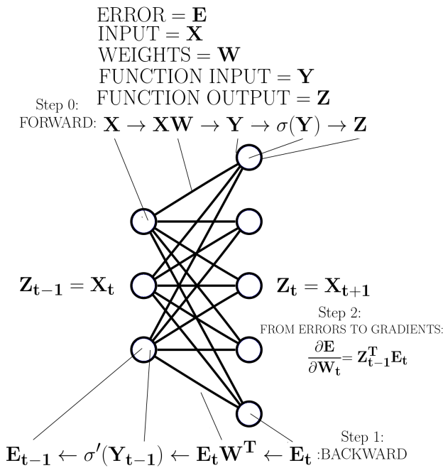
So for each input, we multiply by all weights, and add up all those contributions at the output nodes, or more easily we take the matrix product of the input matrix times the weight matrix. In our example, this would be our 128×3 input matrix multiplied by the 3×5 weight matrix (see Figure 1). We thus receive our output matrix as a result which in this example is of size 128×5. We then use this output matrix, apply the non-linear activation function and treat our resulting output matrix as the input matrix to the next layer. We repeat these steps until we reach the error function. We then apply the error function to see how far the predictions are different from the correct values. We can formulate this whole process of the forward pass, and equivalently the backward pass, by defining simple rules (see Figure 1).
For the forward pass with given input data we go from the first to the last layer according to these rules:
- When we encounter a weight matrix, we matrix multiply by this weight and propagate the result.
- If we encounter a function, we put our current result into the function and propagate the function output as our result.
- We treat outputs of the previous layer as inputs into the next layer
- When we encounter the error function we apply it and thus generate the error for our backward pass
The backward pass for a given error is similar but proceeds from the last to the first layer where the error generated in rule 4 in the forward pass represents the “inputs” to the last layer. We then go backward through the network and follow these rules:
- When we encounter a weight matrix, we matrix multiply by the transpose of the matrix and propagate the result.
- If we encounter a function, we multiply (element-wise) by the derivative of that function with respect to the inputs that this function received from the forward pass. (see Figure 1)
- We treat errors of the previous layer as inputs (errors) into the next layer
To calculate the gradients, we use each intermediate result obtained after executing rule 2 in the backward pass and matrix multiply this intermediate result by the value of rule 2 from the forward pass from the previous layer (see Figure 1).
Additional material: Coursera: Neural Networks for Machine Learning: The Backpropagation Learning Procedure
Rectified Linear Function
The rectified linear function is a simple non-linearity: It evaluates to 0 for negative inputs, and positive values remain untouched (f(x) = max(0,x)). The gradient of the rectified linear function is 1 for all positive values and 0 for negative values. This means that during backpropagation, negative gradients will not be used to update the weights of the outgoing rectified linear unit.
However, because we have a gradient of 1 for any positive value we have much better training speed when compared to other non-linear functions due to the good gradient flow. For example, the logistic sigmoid function has very tiny gradients for large positive and negative values so that learning nearly stops in these regions (this behavior is similar to a saddle point).
Despite the fact that negative gradients do not propagate with rectified linear functions (the gradient is zero here), large gradients for positive values are very powerful and ensure fast training regardless of the size of the gradient. Once these benefits were discovered, rectified linear functions and similar activation functions with large gradients became the activation functions of choice for deep networks.
Momentum / Nesterov’s Accelerated Gradient
Momentum uses the idea that the gradient zigzags every now and then but generally follows a rather straight line towards a local minimum. As such, if we move faster in this general direction and disregard the zigzag directions we will arrive faster at the local minimum, in general.
To realize this behavior we keep track of a running momentum matrix, which is the weighted running sum of the gradient, and we add that momentum matrix value to the gradient. The size of this momentum matrix is kept in check by attenuating it on every update (multiply by a momentum value between 0.7-0.99). Over time, the zigzag dimensions will be smoothed out in our running momentum matrix: A zig in one direction and a zag in the exact opposite direction cancel out and yield a straight line towards the general direction of the local minimum. In the beginning, the general direction towards the local minimum is not strongly established (a sequence of zags with no zigs, or vice versa), and the momentum matrix needs to be attenuated more strongly or the values for the momentum increasingly emphasize zigzagging directions, which in turn can lead to unstable learning. Thus, the momentum value should be kept small (0.5-0.7) in the beginning when no general direction towards a local minimum has been established. Later the momentum value can be increased rapidly (0.9-0.999).
Usually, the gradient update is applied first, and then the jump into the momentum direction follows. However, Nesterov showed that it is better to first jump into the momentum direction and then correct this direction with a gradient update; this procedure is known as “Nesterov’s accelerated gradient” (sometimes “Nesterov momentum”) and yields faster convergence to a local minimum.
Additional material: Coursera: Neural Networks for Machine Learning: 3. The Momentum Method
RMSprop (Root Mean Square Propagation)
RMSprop keeps track of the weighted running mean of the squared gradient and then divides each calculated gradient by the square root of this weighted running mean (it essentially normalizes the gradient by dividing by the magnitude of recent gradients). The consequence is that when a plateau in the error surface is encountered and the gradient is very small, the updates take greater steps, ensuring faster learning (a small update: 0.00001, the square root of the weighted average: 0.00005, update size: 0.2). On the other hand, RMSprop protects against exploding gradients (a large update: 100, the square root of the weighted average: 25, update size: 4) and is thus used frequently in recurrent neural networks and LSTMs to protect both against vanishing and exploding gradients.
Additional material:
Coursera: Neural Networks for Machine Learning for Machine Learning: RMSProp
Additional animations comparing different optimization problems.
Dropout
Imagine you (a unit in a convolutional network) are preparing for an exam (a classification task) and you know that during the exam you are permitted to copy answers from your peers (other units). Will you study for the exam? The answer to this question is probably yes or no depending on whether at least some students in your class have studied for the exam.
Let’s say you know that there are two students (units) in your class (convolutional net) who have the reputation of studying for every exam they take (every image that is presented). So you do not study for the exam and just copy from these students (you weigh the input from a single “elite” unit in the previous layer highly).
Now we introduce an infectious flu (dropout) that affects 50% of all students. Now there is a high chance that these two students who actually studied for the exam will not be present, so relying on copying their answers is no longer a good strategy. So this time you have to learn by yourself (make choices which take into account all units in a layer and not just the elite units).
In other words, dropout decouples the information processing of units so that they cannot rely on some unit “superstars” which always seem to have the right answer (these superstars detect features which are more important than the features that other units detect).
This in turn democratizes the classification process so that every unit makes computations that are largely independent of strong influencers, and thus reduces bias by ensuring less extreme opinions (there are no mainstream opinions). This decoupling of units in turn leads to strong regularization and better generalization (wisdom of the crowd).
L1 and L2 Regularization
L1 and L2 regularization penalizes the size of the weights of a network so that large output values that signify strong confidence can no longer be achieved from a single large weight, but instead require several medium-sized weights. Since many units have to agree to achieve a large value, it is less likely that the output will be biased by the opinion of a single unit. Conceptually, it penalizes strong opinions from single units and encourages taking into account the opinion of multiple units, thus reducing bias.
The L1 regularization penalizes the absolute size of the weight, while the L2 penalizes the squared size of the weight. This penalty is added to the error function value thus increasing the error if larger weights are used. As a result, the network is driven to solve the problem with small weights.
Since even small weights produce a sizeable L1 penalty, the L1 penalty has the effect that most weights will be set to zero while a few medium-to-large weights remain. Because fewer non-zero weights exist, the network must be highly confident about its results to achieve good predictive performance.
The L2 penalty encourages very small non-zero weights (large weight = very large error). Here the prediction is made by almost all weights thus reducing the bias (there are no influencers that can turn around outcomes by themselves).
Additional material: Coursera: Neural Networks for Machine Learning: 2. Limiting the Size of the Weights
Conclusion to Part 2
This concludes part 2 of this crash course on deep learning. Please check back soon for the next part of the series. In part 3, I’ll provide some details on learning algorithms, unsupervised learning, sequence learning, and natural language processing, and in part 4 I’ll go into reinforcement learning. In case you missed it, be sure to check out part 1 of the series.
Meanwhile, you might be interested in learning about cuDNN, DIGITS, Computer Vision with Caffe, Natural Language Processing with Torch, Neural Machine Translation, the Mocha.jl deep learning framework for Julia, or other Parallel Forall posts on deep learning.