This series of blog posts aims to provide an intuitive and gentle introduction to deep learning that does not rely heavily on math or theoretical constructs. The first part of this series provided an overview of the field of deep learning, covering fundamental and core concepts. The second part of the series provided an overview of training neural networks efficiently and gave a background on the history of the field. In this post, we’ll look at sequence learning with a focus on natural language processing. Part 4 of the series covers reinforcement learning.
Sequence Learning
Everything in life depends on time and therefore, represents a sequence. To perform machine learning with sequential data (text, speech, video, etc.) we could use a regular neural network and feed it the entire sequence, but the input size of our data would be fixed, which is quite limiting. Other problems with this approach occur if important events in a sequence lie just outside of the input window. What we need is (1) a network to which we can feed sequences of arbitrary length one element of the sequence per time step (for example a video is just a sequence of images; we feed the network one image at a time); and (2) a network which has some kind of memory to remember important events which happened many time steps in the past. These problems and requirements have led to a variety of different recurrent neural networks.
Recurrent Neural Networks
If we want a regular neural network to solve the problem of adding two numbers, then we could just input the two numbers and train the network to prediction the sum of these outputs. If we now have three instead of two numbers which we want to add we could (1) extend our network with additional input and additional weights and retrain it, or (2) feed the output, that is the sum, of the first two numbers along with the third number back into the network. Approach (2) is clearly better because we can hope that the network will perform well without retraining the entire network (the network already “knows” how to add two numbers, so it should know how to add a sum of two numbers and another number). If we are instead given the task of first adding two numbers and then subtracting two different numbers, this approach would not work anymore. Even if we use an additional weight from the output we cannot guarantee correct outputs: it is equivalent to trying to approximate subtraction of two numbers with an addition and a multiplication by a sum, which will generally not work! Instead, we could try to “change the program” from the network from “addition” to “subtraction”. We can do this by weighting the output of the hidden layer, and feed it back into the hidden layer—a recurrent weight (see Figure 2)! With this approach we change the internal dynamics of the network with every new input; that is, at every new number. The network will learn to change the program from “addition” to “subtraction” after the first two numbers and thus will be able to solve the problem (albeit with some errors in accuracy).
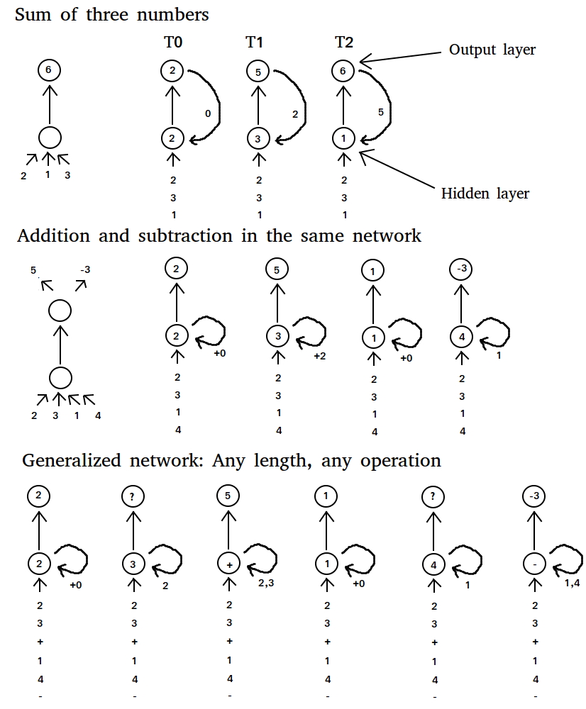
We can even generalize this approach and feed the network with two numbers, one by one, and then feed in a “special” number that represents the mathematical operation “addition”, “subtraction”, “multiplication” and so forth. Although this would not work perfectly in practice, we could get results which are in the ballpark of the correct result. However, the main point here is not getting the correct result, but that we can train recurrent neural networks to learn very specific outputs for an arbitrary sequence of inputs, which is very powerful.
As an example, we can teach recurrent networks to learn sequences of words. Soumith Chintala and Wojciech Zaremba wrote an excellent Parallel Forall blog post about natural language understanding using RNNs. RNNs can also be used to generate sequences. Andrej Karpathy wrote a fascinating and entertaining blog post in which he demonstrated character-level RNNs that can generate imitations of everything from Shakespeare to Linux source code, to baby names.
Long Short-Term Memory (LSTM)
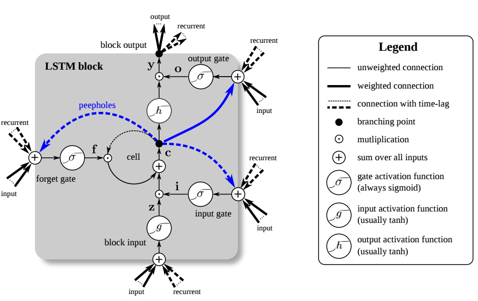
Long short-term memory (LSTM) units use a linear unit with a self-connection with a constant weight of 1.0. This allows a value (forward pass) or gradient (backward pass) that flows into this self-recurrent unit to be preserved indefinitely (inputs or errors multiplied by 1.0 still have same value; thus, the output or error of the previous time step is the same as the output for the next time step) so that the value or gradient can be retrieved exactly at the time step when it is needed most. This self-recurrent unit, the memory cell, provides a kind of memory which can store information which lies dozen of time-steps in the past. This is very powerful for many tasks, for example for text data, an LSTM unit can store information contained in the previous paragraph and apply this information to a sentence in the current paragraph.
Additionally, a common problem in deep networks is the “vanishing gradient” problem, where the gradient gets smaller and smaller with each layer until it is too small to affect the deepest layers. With the memory cell in LSTMs, we have continuous gradient flow (errors maintain their value) which thus eliminates the vanishing gradient problem and enables learning from sequences which are hundreds of time steps long.
However, sometimes we want to throw away information in the memory cell and replace it with newer, more relevant information. At the same time, we do not want to confuse the rest of the network by releasing unnecessary information into the network. To solve this problem, the LSTM unit has a forget gate which deletes the information in the self-recurrent unit without releasing the information into the network (see Figure 1). In this way, we can throw away information without causing confusion and make room for a new memory. The forget gate does this by multiplying the value of the memory cell by a number between 0 (delete) and 1 (keep everything). The exact value is determined by the current input and the LSTM unit output of the previous time step.
At other times, the memory cell contains a that needs to be kept intact for many time steps. To do this LSTM adds another gate, the input or write gate, which can be closed so that no new information flows into the memory cell (see Figure 1). This way the data in the memory cell is protected until it is needed.
Another gate manipulates the output from the memory cell by multiplying the output of the memory cell by a number between 0 (no outputs) and 1 (preserve output) (see Figure 1). This gate may be useful if multiple memories compete against each other: A memory cell might say “My memory is very important right now! So I release it now!” but the network might say: “Your memory is important, true, but other memory cells have much more important memories than you do! So I send small values to your output gate which will turn you off and large values to the other output gates so that the more important memories win!”
The connectivity of an LSTM unit may seem a bit complicated at first, and you will need some time to understand it. However, if you isolate all the parts you can see that the structure is essentially the same as in normal recurrent neural networks, in which inputs and recurrent weights flow to all gates, which in turn are connected to the self-recurrent memory cell.
To dive deeper into LSTM and make sense of the whole architecture I recommend reading LSTM: A Search Space Odyssey and the original LSTM paper.
Word Embedding
Imagine the word “cat” and all other words which closely relate to the word “cat”. You might think about words like “kitten”, “feline”. Now think about words which are a bit dissimilar to the word “cat” but which are more similar to “cat” than, say, “car”. You might come up with nouns like “lion”, “tiger”, “dog”, “animal” or verbs like “purring”, “mewing”, “sleeping” and so forth.
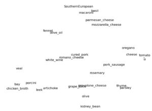
Now imagine a three-dimensional space where we put the word “cat” in the middle of that space. The words mentioned above that are more similar to the word “cat” map to locations closer to the location of “cat” in the space; for example, “kitty” and “feline” are close; “tiger” and “lion” are a bit further away; “dog” further still; and “car” is very, very far away. See Figure 3 for an example of words in cooking recipes and their word embedding space in two dimensions.
If we use vectors that point to each word in this space, then each vector will consists of 3 coordinates which give the position in this space, e.g. if “cat” is (0,0,0) then “kitty” might have the coordinates (0.1,0.2,-0.3) while car has the coordinates (10,0,-15).
This space is then a word embedding space for our vocabulary (words) above and each vector with 3 coordinates is a word embedding which we can use as input data for our algorithms.
Typically, an embedding space contains thousands of words and more than a hundred dimensions. This space is difficult to comprehend for humans, but the property that similar words lie close together in the embedding space still holds. For machines, this is an excellent representation for words which improves results for many tasks that deal with language.
If you want to learn more about word embedding and see how we can apply them to create models which can “understand” language (at least to a certain degree), I recommend you to read Understanding Natural Language with Deep Neural Networks Using Torch by Soumith Chintala and Wojciech Zaremba.
Encoder-Decoder
Stop for a moment and imagine a tomato. Now think about ingredients or dishes that go well with tomatoes. If your thinking is similar to the most common recipes that you find online, then you should have thought about ingredients such as cheese and salami (pizza); parmesan, basil, macaroni; and other ingredients such as olive oil, thyme, and parsley. These ingredients are mostly associated with Italian and Mediterranean cuisines.
Now think about the same tomato but in terms of Mexican cuisine. You might associate the tomato with beans, corn (maize), chilies, cilantro, or avocados.
What you just did was to transform the representation of the word “tomato” into a new representation in terms of “tomato in Mexican cuisine”.
You can think of the encoder doing the same thing. It takes input word by word and transforms it into a new “thought vector” by transforming the representation of all words accordingly (just like adding the context “Mexican cuisine” to “tomato”). This is the first step of the encoder-decoder architecture.
The second step in the encoder-decoder architecture exploits the fact that representations of two different languages have similar geometry in the word embedding space even though they use completely different words for a certain thing. For example, the word cat in German is “Katze” and the word dog is “Hund”, which are of course different words, but the underlying relationships between these words will be nearly the same, that is Katze relates to Hund as cat relates to dog such that the difference in “thought vectors” between Katze and Hund, and cat and dog will be quite similar. Or in other words, even though the words are different they describe a similar “thought vector”. There are some words which cannot be really expressed in another language, but these cases are rare and in general the relationships between words should be similar.
With these ideas, we can now construct a decoder network. We feed our generated “thought vectors” from our English encoder word by word into the German decoder. The German decoder reinterprets these “thought vectors” or “transformations of relationships” as belonging to the “German word vector space”, and thus will produce a sentence which captures the same relationships as the English sentence, but in terms of German words. So we essentially construct a network that can translate languages. This idea is still developing in current research; results are not perfect, but they are rapidly improving and soon this method might be the best way to translate languages.
If you would like to dive deeper into the encoder-decoder architecture and Neural Machine Translation, I recommend you read this comprehensive Parallel Forall blog post about the encoder-decoder architecture by Kyunghyun Cho.
Conclusion
We have seen that we can use recurrent neural networks to solve difficult tasks which deal with sequences of arbitrary length. We have also seen that memory of past input is crucial for successful sequence learning and that LSTMs provide improved performance in this case and alleviate the vanishing gradient problem. We delved into word-embeddings and how we can use them to train recurrent architectures to acquire a certain sense of language understanding.
I hope you enjoyed this blog post. Stay tuned for the next post in this series which will deal with reinforcement learning. If you have any questions please post them in the comments below and I will answer them. Be sure to read part 1, part 2, and part 4 of the series to learn about deep learning fundamental and core concepts, history, and training algorithms, and reinforcement learning!
To learn even more about deep neural networks, come to the 2016 GPU Technology Conference (April 4-7 in San Jose, CA) and learn from the experts. Register now to save 20% with code “MHarris2603”!