The NVIDIA Deep Learning GPU Training System (DIGITS) puts the power of deep learning in the hands of data scientists and researchers. Using DIGITS you can perform common deep learning tasks such as managing data, defining networks, training several models in parallel, monitoring training performance in real time, and choosing the best model from the results browser. DIGITS is completely interactive so that you can focus on designing and training networks rather than programming and debugging.
DIGITS 4 introduces a new object detection workflow that allows you to train networks to detect objects (such as faces, vehicles, or pedestrians) in images and define bounding boxes around them. See the post Deep Learning for Object Detection with DIGITS for a walk-through of how to use this new functionality.

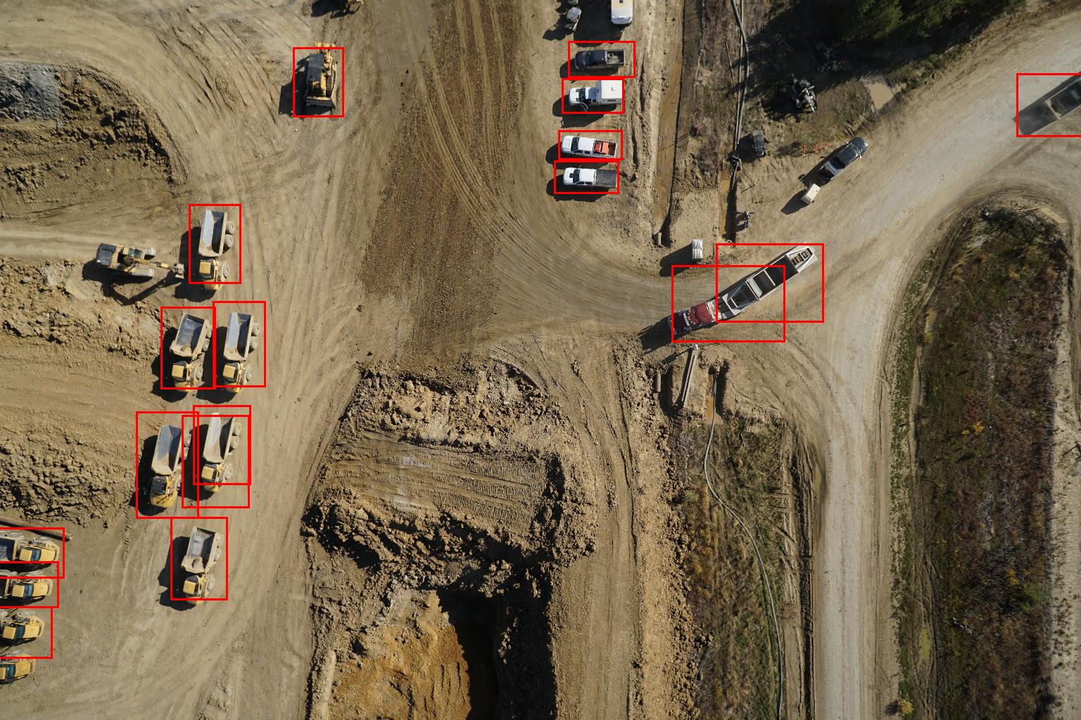
In order to get you up and running as fast as possible with this new workflow, DIGITS now includes a new example neural network model architecture called DetectNet. Figure 1 shows an example of the output of DetectNet when trained to detect vehicles in aerial imagery. DetectNet is provided as a standard model definition in DIGITS 4 and is trained using the Caffe deep learning framework. In this post we will explore the structure of DetectNet and show you how it is trained to perform object detection.
DetectNet Data Format
Image classification training data samples are simply images (usually a small image or patch containing a single object) labeled by class (typically integer class ID or a string class name). Object detection, on the other hand, requires more information for training. DetectNet training data samples are larger images that contain multiple objects. For each object in the image the training label must capture not only the class of the object but also the coordinates of the corners of its bounding box. Because the number of objects can vary between training images, a naive choice of label format with varying length and dimensionality would make defining a loss function difficult.
DetectNet solves this key problem by introducing a fixed 3-dimensional label format that enables DetectNet to ingest images of any size with a variable number of objects present. The DetectNet data representation is inspired by the representation used by [Redmon et al. 2015].
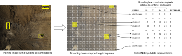
Figure 2 shows the process that DIGITS uses to ingest annotated training images for training DetectNet. DIGITS overlays the image with a regular grid with spacing slightly smaller than the smallest object we wish to detect. Each grid square is labeled with two key pieces of information: the class of object present in the grid square and the pixel coordinates of the corners of the bounding box of that object relative to the center of the grid square. In the case where no object is present in the grid square a special “dontcare” class is used so that the data representation maintains a fixed size. A coverage value of 0 or 1 is also provided to indicate whether an object is present within the grid square. In the case where multiple objects are present in the same grid square DetectNet selects the object that occupies the most pixels within the grid square. In the case of a tie the object with the bounding box with the lowest y-value is used. This choice is arbitrary for aerial imagery but is beneficial for datasets with a ground-plane, such as automotive cameras, where a bounding box with lower y-value indicates an object that is closer to the camera.
The training objective for DetectNet is to predict this data representation for a given image; in other words, for each grid square DetectNet must predict whether an object is present and where the bounding box corners for that object are relative to the center of the grid square.
DetectNet Architecture
The DetectNet architecture has five parts specified in the Caffe model definition file. Figure 3 shows the DetectNet architecture used during training, pointing out three important processes.
- Data layers ingest the training images and labels and a transformer layer applies online data augmentation.
- A fully-convolutional network (FCN) performs feature extraction and prediction of object classes and bounding boxes per grid square.
- Loss functions simultaneously measure the error in the two tasks of predicting the object coverage and object bounding box corners per grid square.
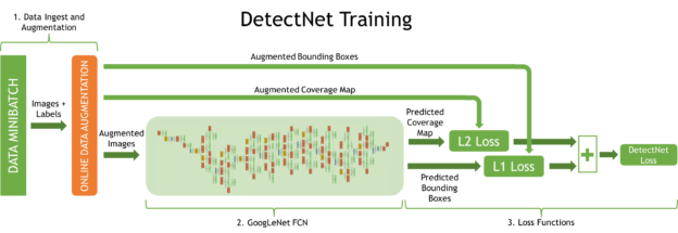
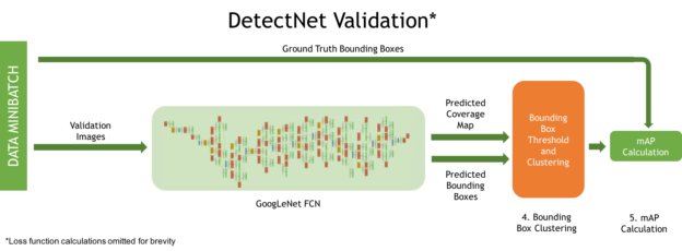
Figure 4 shows the DetectNet architecture during validation, and two more key processes.
- A clustering function produces the final set of predicted bounding boxes during validation.
- A simplified version of the mean Average Precision (mAP) metric is computed to measure model performance against the validation dataset.
You can specify the spacing of the grid squares in the training labels by setting the stride in pixels in the detectnet_groundtruth_param layer. For example:
detectnet_groundtruth_param {
    stride: 16
    scale_cvg: 0.4
    gridbox_type: GRIDBOX_MIN
    min_cvg_len: 20
    coverage_type: RECTANGULAR
    image_size_x: 1024
    image_size_y: 512
    obj_norm: true
    crop_bboxes: false
  }
In this layer you can also specify an image training patch size (image_size_x, image_size_y). When these parameters are set, every time an image is fed into DetectNet during training it takes a random crop of this size as input. This can be useful if you have very large images in which the objects you wish to detect are very small.
The parameters of online data augmentation are defined in the detectnet_augmentation_param layer. For example:
detectnet_augmentation_param {
    crop_prob: 1.0
    shift_x: 32
    shift_y: 32
    scale_prob: 0.4
    scale_min: 0.8
    scale_max: 1.2
    flip_prob: 0.5
    rotation_prob: 0.0
    max_rotate_degree: 5.0
    hue_rotation_prob: 0.8
    hue_rotation: 30.0
    desaturation_prob: 0.8
    desaturation_max: 0.8
  }
Data augmentation is essential to successful training of a high sensitivity and accurate object detector using DetectNet. The parameters of detectnet_augmentation_param define the extent to which random transformations like pixel shifts and flips should be applied to training images and labels each time they are ingested. The benefit of using online augmentation is that the network never sees exactly the same training image twice, so it is much more robust to overfitting and natural variance in the appearance of objects in test images than it would be if we used a one-time static augmentation process.
The FCN sub-network of DetectNet has the same structure as GoogLeNet without the data input layers, final pooling layer and output layers [Szegedy et al. 2014]. This has the major benefit of allowing DetectNet to be initialized using a pre-trained GoogLeNet model, thereby reducing training time and improving final model accuracy. An FCN is a convolutional neural network (CNN) with no fully-connected layers. This means that the network can accept input images with varying sizes and effectively applies a CNN in a strided sliding window fashion. The output is a real-valued multi-dimensional array that can be overlaid on the image, much like the DetectNet input labels described above. Using GoogLeNet with it’s final pooling layer removed results in the sliding window application of a CNN with a receptive field of 555 x 555 pixels and a stride of 16 pixels.
DetectNet uses a linear combination of two separate loss functions to produce its final loss function for optimization. coverage_loss is the sum of squares of differences between the true and predicted object coverage across all grid squares in a training data sample.

bbox_loss is the mean L1 loss (mean absolute difference) for the true and predicted corners of the bounding box for the object covered by each grid square.
![\frac{1}{2N} \sum_{i=1}^{N}\Big[\big|x_1^t - x_1^p\big|+\big|y_1^t - y_1^p\big|+\big|x_2^t - x_2^p\big|+\big|y_2^t - y_2^p\big|\Big]](https://s0.wp.com/latex.php?latex=%5Cfrac%7B1%7D%7B2N%7D+%5Csum_%7Bi%3D1%7D%5E%7BN%7D%5CBig%5B%5Cbig%7Cx_1%5Et+-+x_1%5Ep%5Cbig%7C%2B%5Cbig%7Cy_1%5Et+-+y_1%5Ep%5Cbig%7C%2B%5Cbig%7Cx_2%5Et+-+x_2%5Ep%5Cbig%7C%2B%5Cbig%7Cy_2%5Et+-+y_2%5Ep%5Cbig%7C%5CBig%5D&bg=transparent&fg=000&s=0&c=20201002)
As its training objective, Caffe minimizes a weighted sum of these loss values.
DetectNet Inference
In the final layers of DetectNet the openCV groupRectangles algorithm is used to cluster and filter the set of bounding boxes generated for grid squares with predicted coverage values greater than or equal to gridbox_cvg_threshold, which is specified in the DetectNet model definition prototxt file. This algorithm clusters bounding boxes using the rectangle equivalence criteria that combines rectangles with similar sizes and locations. The similarity is defined by a variable eps, where a value of zero represents no clustering, and as eps goes to positive infinity, all bounding boxes are combined in one cluster. After clustering, small clusters containing less than or equal to gridbox_rect_thresh rectangles are rejected. For remaining clusters, the average rectangle is computed and put into the output rectangle list. Clustering is implemented in a Python function that is invoked in Caffe through the “Python Layers” interface. The parameters of groupRectangles are specified in the cluster layer in the DetectNet model definition file.
DetectNet also uses the “Python Layers” interface to calculate and output a simplified mean Average Precision (mAP) score for the final set of output bounding boxes. For each predicted bounding box and each ground truth bounding box the Intersection over Union (IoU) score is computed. IoU is the ratio of the overlapping areas of two bounding boxes to the sum of their areas. Using a user-defined IoU threshold (default 0.7), predicted bounding boxes can be designated as either true positives or false positives with respect to the ground truth bounding boxes. If a ground truth bounding box cannot be paired with a predicted bounding box such that the IoU exceeds the threshold, then that bounding box is a false negative—in other words, it represents an undetected object. The simplified mAP score output by DetectNet is the product of precision (ratio of true positives to true positives plus false positives) and recall (ratio of true positives to true positives plus true negatives). It’s a good combined measure for how sensitive DetectNet is to objects of interest, how well it avoids false alarms and how precise it’s bounding box estimates are. Further details about this kind of error analysis can be found in [Hoiem et al. 2012].
Training and Inference Performance
The major benefit of using DetectNet for object detection is the efficiency with which all objects within a large image can be detected and have accurate bounding boxes generated. The use of an FCN within DetectNet is more efficient than using a CNN classifier as a sliding window detector as it avoids redundant computation due to overlapping windows. It is also simpler and more elegant to perform this task with a single neural network architecture rather than a multi-stage algorithmic process.
Training DetectNet on a dataset of 307 training images with 24 validation images, all of size 1536×1024 pixels, takes 63 minutes on a single Titan X in DIGITS 4 with NVIDIA Caffe 0.15.7 and cuDNN RC 5.1.
On a Titan X GPU using NVIDIA Caffe 0.15.7 and cuDNN RC 5.1 DetectNet can carry out inference on these same 1536×1024 pixel images with a grid spacing of 16 pixels in just 41ms (approximately 24 FPS).
Getting started with DetectNet
If you wish to try DetectNet against your own object detection dataset it is available now in DIGITS 4. A walkthrough on how to use the object detection workflow in DIGITS is also provided. Also check out the post Deep Learning for Object Detection with DIGITS for a walk-through of how to use the object detection functionality in DIGITS 4.
If you wish to know more about the pros and cons of different Deep Learning approaches to object detection you can watch Jon Barker’s talk from GTC 2016.
You can find more Deep Learning educational resources, including webinars and hands-on labs, from the NVIDIA Deep Learning Institute.
References
Hoiem, D., Chodpathumwan, Y., and Dai, Q. 2012. Diagnosing Error in Object Detectors. Computer Vision – ECCV 2012, Springer Berlin Heidelberg, 340–353.
Redmon, J., Divvala, S., Girshick, R., and Farhadi, A. 2015. You Only Look Once: Unified, Real-Time Object Detection. arXiv [cs.CV]. http://arxiv.org/abs/1506.02640.
Szegedy, C., Liu, W., Jia, Y., et al. 2014. Going Deeper with Convolutions. arXiv [cs.CV]. http://arxiv.org/abs/1409.4842.