Graphs are mathematical structures used to model many types of relationships and processes in physical, biological, social and information systems. They are also used in the solution of various high-performance computing and data analytics problems. The computational requirements of large-scale graph processing for cyberanalytics, genomics, social network analysis and other fields demand powerful and efficient computing performance that only accelerators can provide. With CUDA 8, NVIDIA is introducing nvGRAPH, a new library of GPU-accelerated graph algorithms. Its first release, nvGRAPH 1.0, supports 3 key graph algorithms (PageRank, Single-Source Shortest Path, and Single-Source Widest Path), and our engineering and research teams are already developing new parallel algorithms for future releases. I’ll discuss one of them in detail in this blog post.
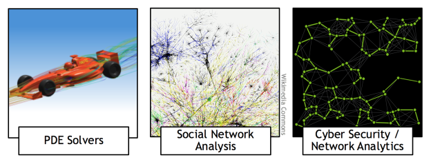
Many applications need to partition graphs into subgraphs, or to find clusters within them. For example, graph partitioning can be used in the numerical solution of partial differential equations (PDEs) to perform more efficient sparse matrix-vector multiplications, and graph clustering can be used to identify communities in social networks and for cybersecurity (see Figure 1).
The quality of graph partitioning or clustering can have a significant impact on the overall performance of an application. Therefore it is very important not only to find the splitting into subgraphs fast by taking advantage of GPUs (our GPU spectral graph partitioning scheme performs up to 7x faster than a CPU implementation), but also to find the best possible splitting, which requires development of new algorithms.
Also, graph partitioning and clustering aims to find a splitting of a graph into subgraphs based on a specific metric. In particular, spectral graph partitioning and clustering relies on the spectrum—the eigenvalues and associated eigenvectors—of the Laplacian matrix corresponding to a given graph. Next, I will formally define this problem, show how it is related to the spectrum of the Laplacian matrix, and investigate its properties and tradeoffs.
Definition
Let a graph 


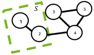
Applications often need to find a splitting of the graph into subgraphs of similar size connected by as few edges as possible. This statement is often formulated as the problem of finding a set of vertices 

where 


For example, a minimum balanced cut of a graph 


It is important to point out that both partitioning and clustering aim to split the original graph into multiple sub-graphs. However, in partitioning the number of partitions and often their size is fixed, while in clustering the fact that there are no partitions can be a result in itself [1]. Also, the optimality of the splitting can be measured by different cost functions, including modularity, betweenness centrality, or flow.
Cost Function
I will focus on the popular ratio and normalized cut cost functions, which are variations of the minimum balanced cut of a graph

and

respectively, where set 


These cost functions are simpler than they look. Notice that the numerator refers to the number of edges cut between partitions and the denominator is related to the number of elements assigned to a particular partition. For example, in distributed sparse matrix-vector multiplication, the numerator relates to the number of elements that must be sent between partitions and the denominator to the work done per partition, measured in terms of the number of rows in the former or number of non-zero elements in the latter equation.
Also, it turns out that it is possible to express these cost functions as

and

where tall matrix ![U=[\textbf{u}_{1},...,\textbf{u}_{p}]](https://s0.wp.com/latex.php?latex=U%3D%5B%5Ctextbf%7Bu%7D_%7B1%7D%2C...%2C%5Ctextbf%7Bu%7D_%7Bp%7D%5D&bg=transparent&fg=000&s=0&c=20201002)


Laplacian Matrix
The Laplacian matrix is defined as 


For example, the Laplacian matrix for the graph

The Laplacian matrix has very interesting properties. To illustrate it, let the set 


This illustrates why in the previous section I could express all the terms in the ratio and normalized cost functions in terms of vector
Key Idea of Spectral Scheme
Notice that obtaining the minimum of the cost function by finding the best non-zero discrete values for the vector 
The key idea of spectral partitioning and clustering is not to look for the discrete solution directly, but instead to do it in two steps.
First, relax the discrete constraints and let vector 
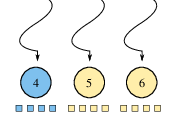
Second, map the obtained real values back to the discrete ones to find the solution of interest. This step can be done using simple heuristics, such as sorting and looking for a gap in the real values, or using more advanced multi-dimensional algorithms, such as the k-means algorithm. In the former case all real values in between gaps, while in the latter case all real values clustered around a particular centroid, will be assigned the same discrete value and therefore will belong to the same particular partition or cluster.
There is no guarantee that the two-step approach will find the best solution, but in practice it often finds a good enough approximation and works reasonably well.
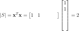
Figure 3 provides a visual outline of the process and Algorithm 1 presents the algorithm in pseudocode.
Let G=(V,E) be an input graph
Let A be the adjacency matrix of G
Let diagonal matrix D = diag(Ae)
Set the Laplacian matrix L=D-A
Solve the eigenvalue problem L u = λu
Use heuristics to transform real into discrete values
Eigenvalue Problem
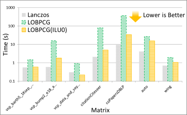
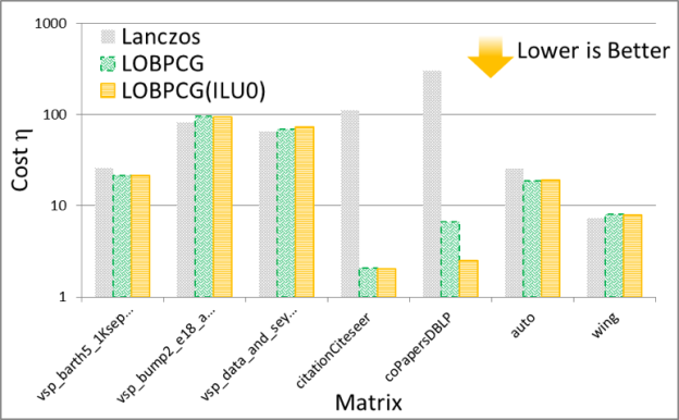
The solution of the eigenvalue problem is often the most time consuming part of spectral graph partitioning /clustering. There are many eigenvalue solvers that can be used to solve it, including Lanczos, Tracemin, Jacobi-Davidson and LOBPCG. In particular, Figures 3 and 4 show experimental results comparing the performance and quality, respectively, of the Lanczos and LOBPCG methods when looking for the 30 smallest eigenvectors of a few matrices from the DIMACS graph collection. Although Lanczos is often the fastest eigenvalue solver, when incomplete-LU with 0 fill-in (ILU0) is available, the preconditioned LOBPCG eigenvalue solver can be competitive and often computes a superior-quality solution.
Experiments
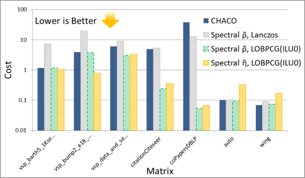
Now I’ll compare the spectral scheme on the GPU with the spectral scheme implemented on the CPU in the CHACO software package. The experiments are performed on a workstation with a 3.2 GHz Intel Core i7-3930K CPU and an NVIDIA Tesla K40c GPU.
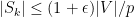
The schemes are very similar, but not identical because CHACO has a slightly different implementation of the algorithms, and also attempts to provide a load-balanced cut within a fixed threshold 
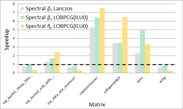
Figures 5 and 6 show the performance and quality of both spectral schemes, respectively. Notice that the GPU spectral scheme using Lanczos often obtains the solution faster, but with variable quality compared to the CPU spectral scheme in CHACO, which also uses a variation of the Lanczos method. On the other hand when using preconditioned LOBPCG the GPU implementation is usually faster, and most of the time obtains a higher quality solution as measured by the cost functions. The detailed results of these experiments can be found in our technical report [2].
Finally, as mentioned earlier there exist many different partitioning and clustering strategies. In particular, some of the popular approaches for providing a balanced cut of a graph use multi-level schemes, implemented in software packages such as METIS. Both spectral and multi-level schemes are global methods that work on the entire graph, in contrast to local heuristics, such as the Kernighan-Lin algorithm.
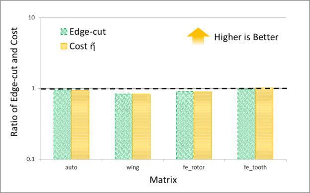
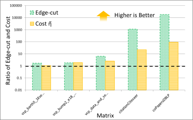
It is interesting to compare the quality of spectral and multi-level schemes in terms of the the edge-cut and cost function obtained by them. The numerical experiments shown in Figures 7 and 8 plot the ratio of these quantities (the cost obtained by METIS divided by the cost obtained by the GPU spectral scheme), for 30 partitions. The result trends indicate that the behavior of the spectral and multi-level schemes is starkly different for two classes of problems: (i) meshes arising from discretization of PDEs and (ii) social network graphs that often have power-law-like distributions of edges per node. My conjecture is that the difference in quality between these schemes results from the fact that multi-level schemes often rely on local information to construct a graph hierarchy that is used to partition the graph.
Notice that for PDEs the quality of the partitioning obtained by both schemes is essentially the same, while for networks with high degree nodes, such as social networks, spectral schemes can obtain significantly higher quality partitions. Even though in our experiments the time taken by the spectral schemes is often larger than that taken by the multi-level schemes, I think that spectral schemes can be a good choice in applications where quality is important. For example, in sparse linear algebra applications, even modest improvements in the quality of partitioning can lead to a significant impact on the overall application performance, so the extra partitioning cost of a spectral scheme may be worthwhile.
Conclusion
I hope that after reading this blog post you have learned some of the intuition behind the spectral graph partitioning/clustering scheme and how it compares to other similar algorithms. A more formal treatment of the subject, with precise derivation of the theoretical results and detailed numerical experiments, can be found in our technical report [2].
The numerical experiments show that spectral partitioning on GPUs can outperform spectral partitioning on the CPU by up to 7x. Also, it is clear that multi-level schemes are a good choice for partitioning meshes arising from PDEs, while spectral schemes can achieve high quality partitioning and clustering on network graphs with high-degree nodes, such as graphs of social networks.
If you need to accelerate graph algorithms in your applications, check out the new GPU-accelerated nvGRAPH library. You can also read more about nvGRAPH in the post “CUDA 8 Features Revealed”. We are considering adding spectral partitioning to nvGRAPH in the future. Please let us know in the comments if you would find this useful.
A Note on Drawing Graphs
Finally, note that eigenvectors of the Laplacian matrix have many other applications. For example, they can be used for drawing graphs. In fact, the graph drawings in this blog were done with them. The interpretation of eigenvectors for this application has been studied in [3].
References
[1] M.E.J. Newman, “Modularity and Community Structure in Networks”, Proc. National Academy of Science, Vol. 103, pp. 8577–8582, 2006.
[2] M. Naumov and T. Moon, “Parallel Spectral Graph Partitioning”, NVIDIA Research Technical Report, NVR-2016-001, March, 2016.
[3] Y. Koren, “Drawing Graphs by Eigenvectors: Theory and Practice”, Computers & Mathematics with Applications, Vol. 49, pp. 1867–1888, 2005.