Linear solvers are probably the most common tool in scientific computing applications. There are two basic classes of methods that can be used to solve an 
Broadly speaking, multi-grid methods can be differentiated into more general algebraic multi-grid (AMG) and the specialized geometric multi-grid (GMG). AMG is a perfect “black-box” solver for problems with unstructured meshes, where elements or volumes can have different numbers of neighbors, and it is difficult to identify a subproblem. There is an interesting blog post demonstrating that GPU accelerators show good performance in AMG using the NVIDIA AmgX library. GMG methods are more efficient than AMG on structured problems, since they can take advantage of the additional information from the geometric representation of the problem. GMG solvers have significantly lower memory requirements, deliver higher computational throughput and also show good scalability. Moreover, these methods require less tuning in general and have a simpler setup than AMG. Let’s take a closer look at GMG and see how well it maps to GPU accelerators.
First of all, it is important to select a modern reference code for GMG. For my case study I chose the HPGMG benchmark. It is a well-established open-source benchmark designed as a proxy for production finite-volume based geometric multi-grid linear solvers. HPGMG was developed by Lawrence Berkeley National Laboratory and is used as a proxy for adaptive mesh refinement combustion codes like the Low Mach Combustion Code. The benchmark solves variable-coefficient elliptic problems using the finite volume method and full multi-grid. It supports high-order discretizations, and is extremely fast and accurate, so it’s a great reference implementation for my case study. It’s worth noting that HPGMG has also been used as an alternative to Linpack for Top500 supercomputer benchmarking; it challenges various aspects of the system and provides a realistic workload for HPC applications.
Why a Hybrid Implementation is Important
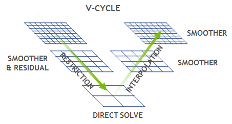
At the core of every multi-grid solver there is a V-cycle computation pattern, shown in Figure 1. A V-cycle starts with the finest structured grid, where a smoothing operation is applied to reduce high-frequency errors, then the residual is calculated and propagated to the coarser grid. This process is repeated until the bottom level is reached, at which point the coarsest problem is solved directly, and then the solution is propagated back to the finest grid. The V-cycle is mainly dominated by the smoothing and residual operations at the top levels. These are usually 3D stencil operations on a structured grid in the case of GMG, or, correspondingly, sparse matrix-vector multiplications for AMG.
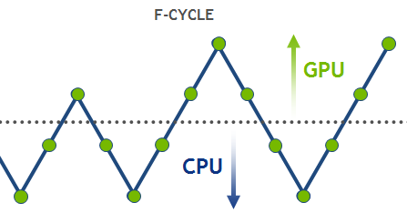
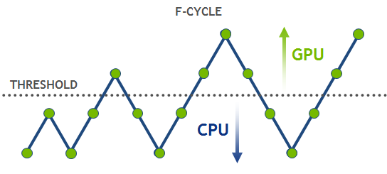
HPGMG implements an F-cycle, which starts at the bottom of the multi-grid hierarchy and performs multiple V-cycles, gradually adding finer levels (see Figure 2). The F-cycle is considered a state-of-the-art in multi-grid methods and converges much faster than a conventional V-cycle.
Let’s discuss how the multi-grid implementation can be mapped to various architectures. Top (fine) levels have lots of grid points and can run efficiently on throughput-oriented parallel architectures like the GPU. On the other hand, bottom (coarse) levels will be latency limited on a GPU because there is not enough work to make efficient use of all the parallel cores. GPUs are not designed to optimize short latency-limited computations. Future GPU architectures will require even more parallelism to fully utilize all available streaming multiprocessors and saturate increased memory bandwidth. The coarse levels problem is not a significant bottleneck for a V-cycle alone, where every coarse level is visited at most twice. However, the cost of coarse levels is significant in an F-cycle, where the coarse levels are visited progressively more often than the fine levels. These coarse grids are better suited for latency-optimized processors like CPUs. Thus, for optimal performance, a hybrid scheme is required to guarantee that each level is executed on the suitable architecture. A possible approach here is to select an empirical threshold for grid size and assign the levels above the threshold to the GPU, and the rest of them to the CPU. Figure 3 shows performance curves for a hybrid implementation of HPGMG v0.3 for larger (h) and smaller (2h) problem sizes using NVIDIA Tesla K40 and dual-socket Intel Xeon E5-2690 v2.
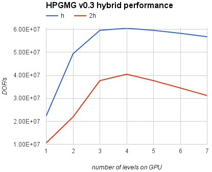
For this system configuration it’s best to keep only the first 4 levels on the GPU and then switch over to the CPU for level 5 and higher. This technique can increase performance by 7% (h) or 30% (2h) compared to running all levels exclusively on the GPU. At the same time, the hybrid implementation achieves up to 4x speed-up compared to the CPU-only version.
Now that both CPU and GPU processors are involved in the computation, it is crucial to discuss memory management.
The Power of Unified Memory
Unified Memory was introduced in CUDA 6 to simplify memory management for GPU developers. Instead of explicit allocation and management of CPU and GPU copies of the same data, Unified Memory creates a shared pool of automatically managed memory that is accessible to both CPU and GPU. You can use a single pointer in both CPU functions and GPU kernels. CPU and GPU memories are physically separate, so the system automatically migrates data between processors. This allows developers to focus on optimizing kernels instead of manipulating memory transfers and managing duplicate copies of the same data.
In HPGMG, Unified Memory enabled a more natural integration of the GPU implementation. I used it to preserve the same data structures and pointers used by the existing implementation and avoid any explicit deep copies of the data. This provides significant benefits for future code maintenance, since any change to the high-level algorithm or the data organization in the CPU code will be automatically reflected in the GPU code. Only a few modifications were made to the original code to enable GPU acceleration: adding corresponding GPU kernels for low-level stencil operators and updating allocations to use cudaMallocManaged() instead of malloc(). Unified Memory simplified the integration of the hybrid scheme, as the following code sample shows.
void smooth(level_type *level,...){
  ...
  if(level->use_cuda) {
    // run on GPU
    smooth_kernel<<<>>>(level, ...);
  }
  else {
    // run on CPU
    #pragma omp parallel for
    for(block = 0; block < num_blocks; block++)
      level->...
  }
}
What about performance? If the data resides on one processor during the critical path of an application, then performance of Unified Memory can be similar to the custom data management (see my OpenACC blog post). This is exactly what we observe operating on the top levels of the V-cycle. However, if there is a lot of data that is shared between CPU and GPU processors, then memory migration can have a significant impact on overall application performance. The Unified Memory page migrations can be more expensive than regular memory copies for current generation GPUs.
In the hybrid multi-grid there are inter-level communications between CPU and GPU levels, such as restriction and interpolation kernels. The same data is accessed by restriction kernels on the GPU and later by a smoothing function on the CPU. This is where the majority of Unified Memory migrations occur. To optimize this phase it is possible to page-lock memory for the first CPU level and map it to both CPU and GPU to avoid expensive migrations (such memory is also called zero-copy). Unfortunately, it is not possible to page-lock memory allocated with cudaMallocManaged(), instead cudaMallocHost() can be used to allocate corresponding data arrays. Note that these arrays will still be accessible from both the CPU and the GPU, but the data will no longer migrate. Figure 4 shows the timelines generated by the NVIDIA Visual Profiler for the full F-cycle, using cudaMallocManaged() (top) and cudaMallocHost() (bottom) for level 5 (all other levels are allocated with cudaMallocManaged() in both cases).
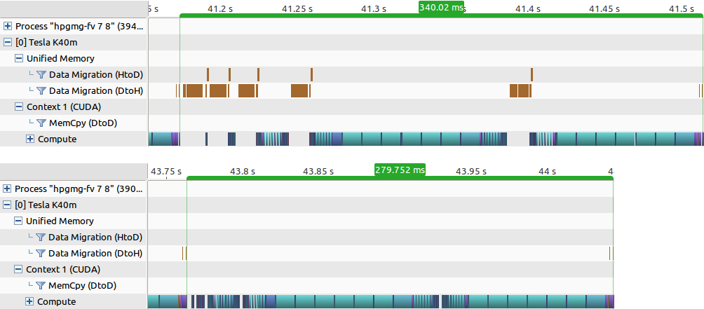
In the case of cudaMallocManaged() the migrations (brown blocks on the timeline in Figure 4) show up every time the threshold line (in Figure 2) between the CPU and GPU is crossed. Since the F-cycle consists of multiple V-cycles of different resolution, the data constantly ping-pongs between CPU and GPU, making up to about 20% of the total time spent on the whole cycle. With the page-locking optimization it is possible to reduce this overhead to almost zero. Importantly, Unified Memory can still be used for everything else. To summarize, my guideline is to use Unified Memory for the majority of your code, and insert custom memory allocations to control the data locality where necessary to maintain high performance of your application. As the performance of Unified Memory improves in the future, the overhead of the migrations in the baseline code will be reduced. Nevertheless, page-locking will still be a useful trick to have in mind when optimizing your Unified Memory applications.
The Future is High-Order Discretizations
The latest version of HPGMG benchmark supports both 2nd and 4th order discretizations for finite-volume methods. The order of the method describes the relationship between grid spacing and error. While differential operators with higher-order discretizations are computationally more complex, they tend to reduce error approximations by several orders of magnitude, which can lead to better convergence in fewer iterations. In a nutshell, the 4th order scheme is much more accurate than the 2nd order scheme for the same memory footprint. These days most production GMG codes use the 2nd order multi-grid. However, the 4th order is being actively explored in many research codes and may become common in the next few years.
The dominant part of the multi-grid is the stencil calculations in the smoother operation, which will be my main focus for performance analysis and optimizations. The 4th-order stencil operations in HPGMG are much more compute-intensive than the seven-point stencil that is used for the 2nd order. More specifically, the 4th-order scheme uses a 25-point stencil with a total of 102 load operations, 214 additions, and 29 multiplications with a flops-to-bytes ratio 4 times higher than the 7-point stencil. The memory footprint is the same in both cases, so this suggests that the higher-order stencils should have more computational work to hide memory latency on the GPU. However, it’s not that simple.
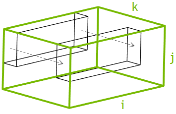
A baseline implementation of the 4th-order smoother involves parallelization over the 2D plane I-J, where each 2D thread block is assigned to a single 3D block from the problem domain and sweeps through the slowest dimension (K), as Figure 5 shows. That is, each thread operates on multiple elements in the K dimension with constant coordinates in the I and J dimensions. The second-order stencil size is relatively small, and in this case the performance is completely dominated by DRAM bandwidth. However, in the 4th-order case the stencil is more complex, so the corresponding kernels generally have low occupancy due to high register usage. This lowers the DRAM bandwidth and shifts the bottleneck to the L2 cache. To improve the performance it is necessary to offload traffic from L2 to faster memories in the streaming multiprocessor, such as registers, caches, and shared memory.
As it turned out, I didn’t have to rewrite every kernel from scratch or significantly change the structure of the code. There are two key optimizations that can be applied to stencils in HPGMG for both 2nd and 4th order, and they help achieve better reuse within the block without disrupting the code. The first optimization caches elements in the slowest K dimension in registers, by restructuring the computation loop to keep track of (k-1), (k), and (k+1) elements as we serially march along the K dimension of the assigned block. This is not a standard optimization provided by the NVCC compiler, which would simply employ registers to store repeated terms at the current loop iteration. The second optimization consists of routing all memory loads for input data through the opt-in L1 cache by using the compiler option -dlcm=ca option, or through the texture cache by using the __ldg() intrinsic. The caches in the SM allow us to save bandwidth going out of the SM when multiple threads in a 2D slice access the same data points during the stencil computation. It is possible to combine these two optimizations together for better performance. Figure 6 demonstrates the resulting 4th-order smoother kernel speed-ups for various optimizations are demonstrated in the following plot.
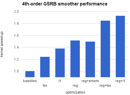
The fastest implementation nearly doubles the performance compared to the baseline. Interestingly, the shared memory version does not provide any advantage and is generally slower than the L1 and texture kernel versions. There is no memory divergence in this code, so implicit caching works much better than the explicit control using shared memory, which involves additional overhead to load data from shared memory to registers. The main goal of all described optimizations is to provide efficient reuse of data in registers and it is likely possible to improve performance even further (for example, using associative reordering). I encourage you to experiment with the code, and don’t hesitate to share your own optimizations.
And It Scales to Thousands of GPUs!
HPGMG is designed to scale well to many processors by decomposing the grid into boxes and distributing them across MPI ranks in a cluster. The GPU implementation can use the same mechanism by assigning each GPU to a single MPI rank. For best results the MPI buffers are allocated with cudaMallocHost() to allow direct writes from the GPU and to enable RDMA between host and network interfaces. In the hybrid approach only the top few levels are running on the GPU, and communications in this case are bandwidth-limited; therefore, the host memory staging can be more efficient than GPUDirect RDMA. Figure 7 shows performance results in DOF/s (degrees of freedom per second) for HPGMG running on the ORNL Titan supercomputer comparing the CPU-only implementation to our hybrid code.
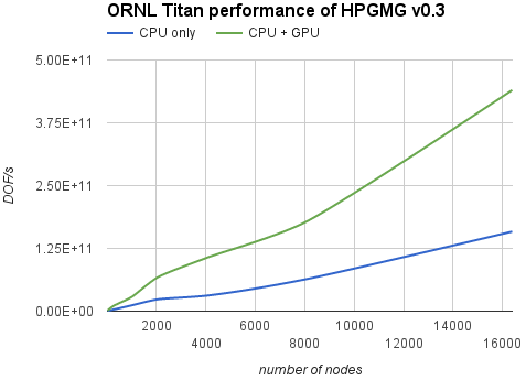
The new hybrid implementation scales linearly and provides a significant boost to overall system performance, up to 2.8x speed-up compared to the CPU-only version. Looking at the official HPGMG performance list from Nov 2015, with GPU acceleration Titan can rise to 2nd place in the rankings.
Attend GTC’16 and Learn More
So far I only talked about multiplicative multi-grid, which is a gold standard in many HPC applications. There is an inherent dependency between levels, which makes it difficult to utilize the GPU on coarse levels and does not allow using both the CPU and GPU simultaneously. Although it is possible to parallelize each smoothing computation by subdividing a grid into a large GPU region and a small CPU region, this method requires many fine-grained inter-processor communications, and it still doesn’t improve the available parallelism in coarse levels. Another interesting approach is called additive multi-grid, where some levels can be processed in parallel and then combined together to remove level dependencies in the V-cycle. Although this method is a great way to overlap fine and coarse levels, it often requires more iterations to converge. In any case, this might be another prospective research direction for multi-grid methods in the near future.
To summarize, in this post I have covered the main algorithm for multi-grid and its hybrid CPU-GPU implementation; discussed the importance of Unified Memory for easier GPU-acceleration of applications and zero-copy optimizations; and touched on a few ideas for improving high-order stencil calculations in GMG.
If you are interested in learning more about multi-grid methods, please attend my talk at the 2016 GPU Technology Conference on Monday April 4th at 11:00am, where I will provide more in-depth GPU analysis of these methods. The full source code for the GPU implementation of the latest HPGMG benchmark v0.3 is available on bitbucket. Feel free to tinker with the code and let me know if you find any bugs or improvements!