Note: This is part two of a detailed three-part series on machine translation with neural networks by Kyunghyun Cho. You may enjoy part 1 and part 3.
In my previous post, I introduced statistical machine translation and showed how it can and should be viewed from the perspective of machine learning: as supervised learning where the input and output are both variable-length sequences. In order to introduce you to neural machine translation, I spent half of the previous post on recurrent neural networks, specifically about how they can (1) summarize a sequence and (2) probabilistically model a sequence. Based on these two properties of recurrent neural networks, in this post I will describe in detail an encoder-decoder model for statistical machine translation.
Encoder-Decoder Architecture for Machine Translation
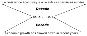
I’m not a neuroscientist or a cognitive scientist, so I can’t speak authoritatively about how the brain works. However, if I were to guess what happens in my brain when I try to translate a short sentence in English to Korean, my brain encodes the English sentence into a set of neuronal activations as I hear them, and from those activations, I decode the corresponding Korean sentence. In other words, the process of (human) translation involves the encoder which turns a sequence of words into a set of neuronal activations (or spikes, or whatever’s going on inside a biological brain) and the decoder which generates a sequence of words in another language, from the set of activations (see Figure 1).
This idea of encoder-decoder architectures is the basic principle behind neural machine translation. In fact, this type of architecture is at the core of deep learning, where the biggest emphasis is on learning a good representation. In some sense, you can always cut any neural network in half, and call the first half an encoder and the other a decoder.
Starting with the work by Kalchbrenner and Blunsom at the University of Oxford in 2013, this encoder-decoder architecture has been proposed by a number of groups, including the Machine Learning Lab (now, MILA) at the University of Montreal (where I work) and Google, as a new way to approach statistical machine translation [Kalchbrenner and Blunsom, 2013; Sutskever et al., 2014; Cho et al., 2014; Bahdanau et al., 2015]. (There is also older, related work by Mikel Forcada at the University of Alcante from 1997! [Forcada and Neco, 1997].) Although there is no restriction on which particular type of neural network is used as either an encoder or a decoder, I’ll focus on using a recurrent neural network for both.
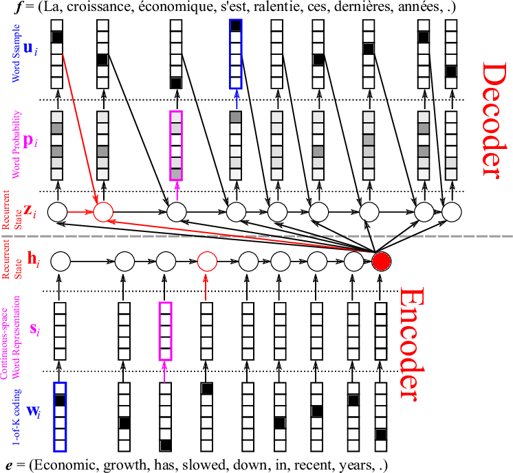
Let’s build our first neural machine translation system! But, before I go into details, let me first show you a big picture of the whole system in Figure 2. Doesn’t it look scarily complicated? Nothing to worry about, as I will walk you through this system one step at a time.
The Encoder
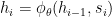
We start from the encoder, a straightforward application of a recurrent neural network, based on its property of sequence summarization. If you recall the previous post, this should be very natural. In short, we apply the recurrent activation function recursively over the input sequence, or sentence, until the end when the final internal state of the RNN 
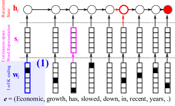
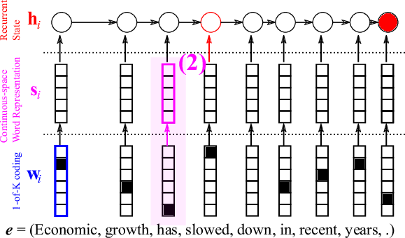
First, each word in the source sentence is represented as a so-called one-hot vector, or 1-of-K coded vector as in Figure 3. This kind of representation is the dumbest representation you can ever find. Every word is equidistant from every other word, meaning that it does not preserve any relationships among them.

We take a hierarchical approach to extracting a sentence representation, a vector that summarizes the input sentence. In that hierarchy, the first step is to obtain a meaningful representation of each word. But, what do I mean by “meaningful” representation? A short answer is “we let the model learn from data!”, and there isn’t any longer answer.
The encoder linearly projects the 1-of-K coded vector 


At this point, we have transformed a sequence of words into a sequence of continuous vectors 
I can write this process of summarization in mathematical notation as
where 

What does the summary vector look like?
Now that we have a summary vector, a natural question comes to mind: “what does this summary vector look like?” I would love to spend hours talking about what that summary vector should look like, what it means and how it’s probably related to representation learning and deep learning, but I think one figure from [Sutskever et al., 2014] says it all in a much more compact form (Figure 6).
To plot the points in Figure 6, Sutskever et al. (2014) trained a neural machine translation system which we’re now training on a large parallel corpus of English and French. Once the model was trained on the corpus, he fed in several English sentences into the encoder to get their corresponding sentence representations, or summary vectors
Unfortunately, human beings are pretty three dimensional, and our screens and papers can only faithfully draw two-dimensional projections. So it’s not easy to show anyone a vector which has hundreds of numbers, especially on paper. There are a number of information visualization techniques for high-dimensional vectors using a much lower-dimensional space. In the case of Figure 6, Sutskever et al. (2014) used principal component analysis (PCA) to project each vector onto a two-dimensional space spanned by the first two principal components (x-axis and y-axis in Figure 6). From this, we can get a rough sense of the relative locations of the summary vectors in the original space. What we can see from Figure 6 is that the summary vectors do preserve the underlying structure, including semantics and syntax (if there’s a such thing as syntax); in other words, similar sentences are close together in summary vector space.
![Figure 6. 2-D Visualization of Sentence Representations from [Sutskever et al., 2014]. Similar sentences are close together in summary-vector space.](/blog/wp-content/uploads/2015/06/Figure6_summary_vector_space.png)
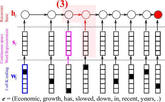
The Decoder
Now that we have a nice fixed-size representation of a source sentence, let’s build a decoder, again using a recurrent neural network (the top half in Figure 2). Again, I will go through each step of the decoder. It may help to keep in mind that the decoder is essentially the encoder flipped upside down.
Let’s start by computing the RNN’s internal state 


The details of 

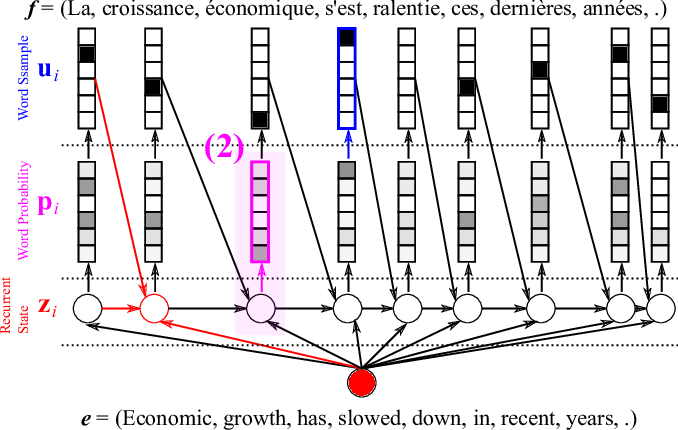
First, we score each word 
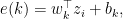
where 

Let’s forget about the bias
Once we compute the score of every word, we now need to turn the scores into proper probabilities using

This type of normalization is called softmax [Bridle, 1990].
Now we have a probability distribution over the target words, which we can use to select a word by sampling the distribution (see here), as Figure 9 shows. After choosing the 

Training: Maximum Likelihood Estimation
Okay, now we have a neural machine translation system ready. How do we train this system so that it can actually translate? As usual with any machine learning model, there are many ways to tune this model to do actual translation. Here, I will describe how to train a neural machine translation model based on the previously described encoder-decoder by maximizing the log-likelihood. Maximum (log-) likelihood estimation (MLE) is a common statistical technique.
First, a so-called parallel corpus 


where 
All we need to do is to maximize this log-likelihood function, which we can do using stochastic gradient descent (SGD).
The gradient of the log-likelihood 
theano.tensor.grad(-loglikelihood, parameters). Here is an example, and here is more detailed documentation.
Once Theano has automatically computed the derivative of the log-likelihood with respect to each parameter, we update the parameter to move along that derivative slowly. Often, this slowly moving part is one that frustrates a lot of people, and this is one of the reasons why many people mistake deep learning for black magic. I agree that finding good learning parameters (initial learning rate, learning rate scheduling, momentum coefficient and its scheduling, and so on) can be frustrating.
So, I often simply go for one of the recently proposed adaptive learning rate algorithms. Among many of them, Adadelta [Zeiler, 2012] and Adam [Kingma and Ba, 2015] are my favourites. They can be easily implemented in Theano, and if you’re not too keen on reading the paper and implementing the algorithm, you can refer to the Theano documentation. Also you might want to have a look at these visualizations of the
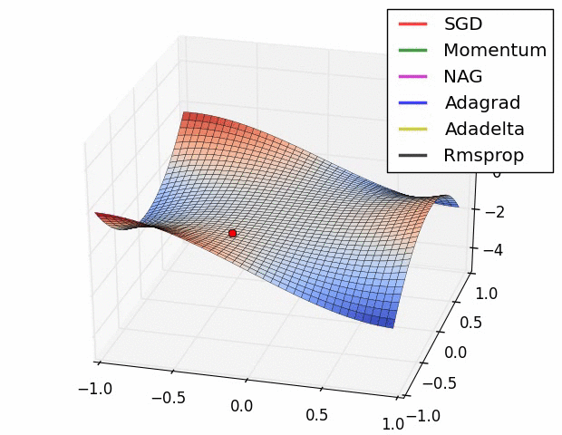
optimization algorithms (also figure 10), although I must warn you that the behavior in this low dimensional space is not necessarily representative of the behavior in a higher dimensional space.
Why GPUs? The Computational Complexity of NMT Training
Does this mean that I can train a neural machine translation model on a large parallel corpus with my laptop? Unfortunately, no. As you may have guessed, the amount of computation you need for each update is quite large, and the number of SGD updates needed to fully train a model is also large. Let’s first count what kind of computation is required for a single forward pass:
- Source word embeddings:
(
source words,
unique words)
- Source embeddings to the encoder:
(
-dim embedding,
recurrent units; two gates and one unit for GRU)
to
:
- Context vector to the decoder:
to
:
- The decoder to the target word embeddings:
(
target words,
-dim target embedding)
- Target embeddings to the output:
(
target words)
- Softmax normalization of the output:

Considering that
Note that most of these computations are matrix-vector or matrix-matrix multiplications of high-dimensional vectors or matrices, and when it comes to Generalized Matrix-Matrix multiplications (GEMM) of large matrices, it’s well-known that GPUs significantly outperform CPUs (in terms of wall-clock time.) So it’s crucial to have a nice set of the latest GPUs to develop, debug and train neural machine translation models.
For instance, see Table 1 for how much time you can save by using GPUs. The table presents only the time needed for translation, and the gap between CPU and GPU grows much greater when training a model, as the complexity estimates above show.
| CPU (Intel i7-4820K) | GPU (GTX TITAN Black) | |
| RNNsearch [Bahadanau et al,, 2015] | 0.09s | 0.02s |
| Table 1. The average per-word decoding/translation time. From [Jean et al., 2015] | ||
I can assure you that I didn’t write this section to impress NVIDIA; you really do need good GPUs to train any realistic neural machine translation models, at least until scalable and affordable universal quantum computers become available!
The Story So Far
Continuing from the previous post, today I described how a recently proposed neural machine translation system is designed using recurrent neural networks. The neural machine translation system in today’s post is a simple, basic model that was recently shown to be excellent in practice for English-French translation.
Based on this basic neural machine translation model, in my next post I will tell you how we can push neural machine translation much further by introducing an attention mechanism into the model. Furthermore, I will show you how we can use neural machine translation to translate from images and even videos into their descriptions! Stay tuned.


![Figure 3. Graphical illustration of different types of recurrent neural networks. From [Pascanu et al., 2014]](https://developer-blogs.nvidia.com/wp-content/uploads/2015/05/Figure_3.png)