This week at GTC 2016, we announced the latest update to NVIDIA Deep Learning SDK, which now includes cuDNN 5. Version 5 offers new features, improved performance and support for the latest generation NVIDIA Tesla P100 GPU. New features in cuDNN 5 include:
-
- Faster forward and backward convolutions using the Winograd convolution algorithm;
-
- 3D FFT Tiling;
-
- Spatial Transformer Networks;
-
- Improved performance and reduced memory usage with FP16 routines on Pascal GPUs;
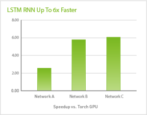
- Support for LSTM recurrent neural networks for sequence learning that deliver up to 6x speedup.
One of the new features we’ve added in cuDNN 5 is support for Recurrent Neural Networks (RNN). RNNs are a powerful tool used for sequence learning in a number of fields, from speech recognition to image captioning. For a brief high-level introduction to RNNs, LSTM and sequence learning, I recommend you check out Tim Dettmers recent post Deep Learning in a Nutshell: Sequence Learning, and for more depth, Soumith Chintala’s post Understanding Natural Language with Deep Neural Networks Using Torch.
I’m excited about the RNN capabilities in cuDNN 5; we’ve put a lot of effort into optimizing their performance on NVIDIA GPUs, and I’ll go into some of the details of these optimizations in this blog post.
cuDNN 5 supports four RNN modes: ReLU activation function, tanh activation function, Gated Recurrent Units (GRU), and Long Short-Term Memory (LSTM). In this case study I’ll look at the performance of an LSTM network, but most of the optimizations can be applied to any RNN.
Step 1: Optimizing a Single Iteration
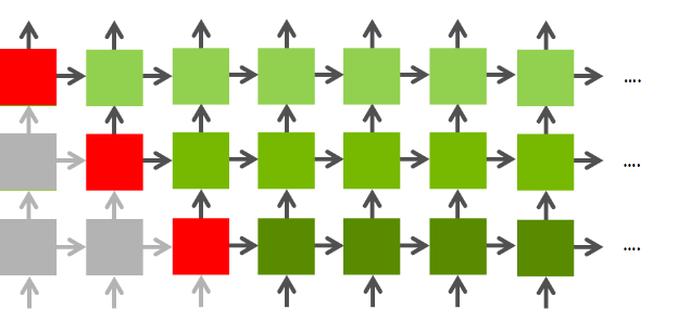
The following equations govern the forward propagation of data through an LSTM unit. Figure 2 shows a diagram of an LSTM unit.


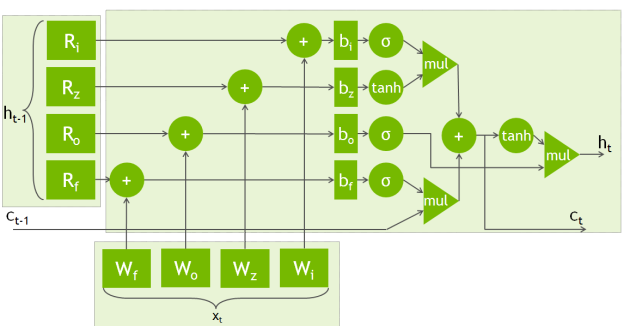
From a computational perspective this boils down to eight matrix-matrix multiplications (GEMMs)—Four with input i, four with input h—and lots of point-wise operations.
The starting point for this case-study is an LSTM implemented operation-by-operation. For each iteration, for each layer, the implementation calls cuBLAS sgemm to perform each of the eight GEMMs, and hand-written CUDA kernels to call each of the point-wise operations. Pseuduocode for the method follows.
for layer in layers:
  for iteration in iterations:
     perform 4 SGEMMs on input from last layer
     perform 4 SGEMMs on input from last iteration
     perform point-wise operations
As a benchmark I measure run time per step, per layer on a Tesla M40 GPU. My benchmark LSTM has 512 hidden units and computes mini batches of size 64. The performance of this baseline implementation is fairly poor, achieving approximately 350 GFLOPS on the M40. The peak performance of this GPU is around 6000 GFLOPs, so there is a lot of room to improve. Let’s get started.
Optimization 1: Combining GEMM Operations
GPUs have very high peak floating-point throughput, but they need a lot of parallelism to approach this peak. The more parallel work you give them, the higher the performance they can achieve. Profiling this LSTM code shows that the GEMM operations use significantly fewer CUDA thread blocks than there are SMs on the GPU, indicating the GPU is massively underused.
GEMM is typically parallelized over the output matrix dimensions, with each thread computing many output elements for maximum efficiency. In this case each of the eight output matrices comprises 512×64 elements, which results in only four thread blocks. Ideally can run significantly more blocks than the GPU has SMs, and to maximize the theoretical occupancy for this kernel at least four blocks per SM (or 96 in total) are needed. (See the CUDA Best Practices guide for more on occupancy.)
If n independent matrix multiplications share the same input, then they can be combined into one larger matrix multiplication with an output n times larger. The first optimization is therefore to combine the four weight matrices operating on the recurrent step into one weight matrix, and to combine the four weight matrices operating on the input into another. This gives us two matrix multiplications instead of eight, but each is four times the size and has four times the parallelism (16 blocks per GEMM). This optimization is fairly common in most framework implementations: it’s a very easy change that leads to a good speedup: the code runs roughly 2x faster.
Optimization 2: Streaming GEMMs
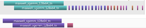
Even with the larger combined GEMMs, performance is still limited by lack of parallelism: there are 16 blocks instead of four, but the target is to have at least 96. The two remaining GEMMs are independent so they can be computed concurrently using CUDA streams. This doubles the number of possible concurrent blocks to 32.
Optimization 3: Fusing Point-wise Operations
Figure 3 shows that now a lot of time is spent in point-wise operations. There’s no need to do these in separate kernels; fusing them into a single kernel reduces data transfers to and from global memory and significantly reduces kernel launch overhead.
At this point I’m fairly happy with the performance of a single iteration: the majority of the computation is in the GEMMs, and they’re exposing as much parallelism as they can. This implementation is about 5x faster than the baseline implementation, but there are more improvements to come.
for layer in layers:
  for iteration in iterations:
     perform sgemm on input from last layer in stream A
     perform sgemm on input from last iteration in stream B
     wait for stream A and stream B
     perform point-wise operations in one kernel
Step 2: Optimizing Many Iterations
In an RNN the operations for a single iteration are repeated many times. This means it’s important to have those operations running efficiently, even if this comes at an upfront cost.
Optimization 4: Pre-Transposing the Weight Matrix
When performing a GEMM the standard BLAS API allows you to transpose either of the two input matrices. Some of the four combinations of transpose/not-transposed run slightly faster or slower than others. Depending on the way that the equations are mapped to the computation, a slower version of the GEMM may be used. By performing a transpose operation up-front on the weight matrix, each step can be made slightly faster. This comes at the cost of the transpose, but that is fairly cheap, so if the transposed matrix is to be used for more than a few iterations it is often worth it.
Optimization 5: Combining Input GEMMs
In many cases all of the inputs are available at the start of the RNN computation. This means that the matrix operations working on these inputs can be started immediately. It also means that they can be combined into larger GEMMs. While at first this may seem like a good thing (there’s more parallelism in the combined GEMMs), propagation of the recurrent GEMMs depends upon the completion of the input GEMMs. So there’s a tradeoff: combining input GEMMs gives more parallelism in that operation, but also prevents overlap with the recurrent GEMMs. The best strategy here depends a lot on the RNN hyperparameters. Combining two input GEMMs works best in this case.
for layer in layers:
  transpose weight matrices
  for iteration in iterations / combination size:
     perform sgemm on combined input from last layer in stream A
     for sub-iteration in combination size:
        perform sgemm on input from last iteration in stream B
        wait for stream A
     wait for stream B
     for sub-iteration in combination size;
        perform pointwise operations in one kernel
Step 3: Optimization with Many Layers
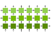
The final step is to consider optimization between layers. Once again, there’s quite a lot of parallelism to be found here. Figure 4 shows the dependency graph for an RNN. As iteration n of a given layer only depends on iteration n-1 of that layer and iteration n of the previous layer it is possible to start on a layer before you’ve finished on the previous layer. This is really powerful: if there are two layers there is twice as much parallelism available.
Going up from one to four layers, throughput increases by roughly 1.7x: from 2.3 TFLOPs to 3.9 TFLOPs. At this point the gains from exposing more parallelism are starting to become more limited. Compared to the original implementation which only had four blocks running at any given time, this implementation can run up to 128 blocks concurrently. This is enough to make use of all of the M40’s resources, achieving nearly 70% of peak floating point performance and running more than 10x faster than the original implementation.
The following table shows the performance achieved after each of the optimizations I have described and the speedup vs. the baseline code.
| Optimization | GFLOPS | Speedup |
| Baseline | 349 | (1.0x) |
| Combined GEMMs | 724 | 2.1x |
| GEMM Streaming | 994 | 2.8x |
| Fused point-wise operations | 1942 | 5.5x |
| Matrix pre-transposition | 2199 | 6.3x |
| Combining Inputs | 2290 | 6.5x |
| Four layers | 3898 | 11.1x |
Backpropagation
Propagating gradients through the backward pass is very similar to propagating values forward. Once the gradients have been propagated the weights can be updated in a single call spanning all iterations: there are no longer any recurrent dependencies. This results in a very large efficient matrix multiplication.
Conclusion
To get the best performance out of Recurrent Neural Networks you often have to expose much more parallelism than direct implementation of the equations provides. In cuDNN we’ve applied these optimizations to four common RNNs, so I strongly recommend that you use cuDNN 5 if you are using these RNNs in your sequence learning application.
For more information:
-
- Watch my GTC 2016 talk, either live Thursday 7th at 14:00 in Room 210H, or via the recording available soon after.
-
- Read our paper describing these methods in more detail on arXiv.
- Download the code used for this blog post on GitHub.
Other resources: