A defining feature of the new Volta GPU Architecture is its Tensor Cores, which give the Tesla V100 accelerator a peak throughput 12 times the 32-bit floating point throughput of the previous-generation Tesla P100. Tensor Cores enable AI programmers to use mixed-precision to achieve higher throughput without sacrificing accuracy.
Tensor Cores are already supported for Deep Learning training either in a main release or via pull requests in many Deep Learning frameworks (including Tensorflow, PyTorch, MXNet, and Caffe2). For more information about enabling Tensor Cores when using these frameworks, check out the Mixed-Precision Training Guide. For Deep Learning inference the recent TensorRT 3 release also supports Tensor Cores.
In this blog post we show you how you to use Tensor Cores in your own application using CUDA Libraries as well as how to program them directly in CUDA C++ device code.
What are Tensor Cores?
Tesla V100’s Tensor Cores are programmable matrix-multiply-and-accumulate units that can deliver up to 125 Tensor TFLOPS for training and inference applications. The Tesla V100 GPU contains 640 Tensor Cores: 8 per SM. Tensor Cores and their associated data paths are custom-crafted to dramatically increase floating-point compute throughput at only modest area and power costs. Clock gating is used extensively to maximize power savings.
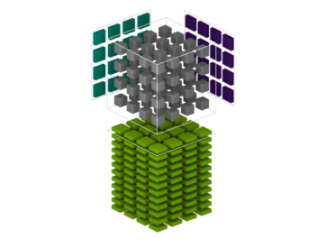
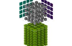
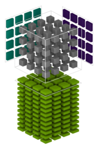
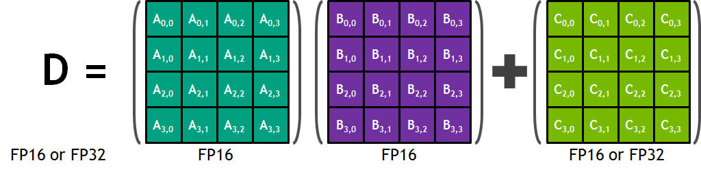
Each Tensor Core provides a 4x4x4 matrix processing array which performs the operation D = A * B + C, where A, B, C and D are 4×4 matrices as Figure 1 shows. The matrix multiply inputs A and B are FP16 matrices, while the accumulation matrices C and D may be FP16 or FP32 matrices.
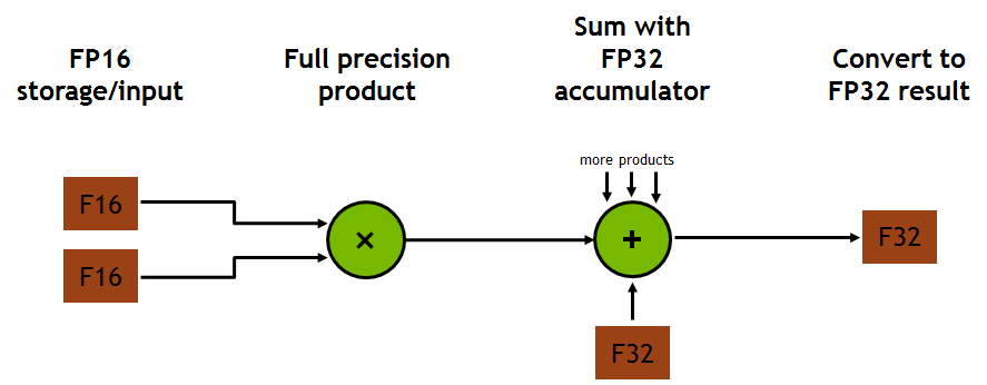
Each Tensor Core performs 64 floating point FMA mixed-precision operations per clock (FP16 input multiply with full-precision product and FP32 accumulate, as Figure 2 shows) and 8 Tensor Cores in an SM perform a total of 1024 floating point operations per clock. This is a dramatic 8X increase in throughput for deep learning applications per SM compared to Pascal GP100 using standard FP32 operations, resulting in a total 12X increase in throughput for the Volta V100 GPU compared to the Pascal P100 GPU. Tensor Cores operate on FP16 input data with FP32 accumulation. The FP16 multiply results in a full-precision result that is accumulated in FP32 operations with the other products in a given dot product for a 4x4x4 matrix multiply, as Figure 8 shows.
During program execution, multiple Tensor Cores are used concurrently by a full warp of execution. The threads within a warp provide a larger 16x16x16 matrix operation to be processed by the Tensor Cores. CUDA exposes these operations as warp-level matrix operations in the CUDA C++ WMMA API. These C++ interfaces provide specialized matrix load, matrix multiply and accumulate, and matrix store operations to efficiently utilize Tensor Cores in CUDA C++ programs.
But before we get into the details of low-level programming of Tensor Cores, let’s look at how to access their performance via CUDA libraries.
Tensor Cores in CUDA Libraries
Two CUDA libraries that use Tensor Cores are cuBLAS and cuDNN. cuBLAS uses Tensor Cores to speed up GEMM computations (GEMM is the BLAS term for a matrix-matrix multiplication); cuDNN uses Tensor Cores to speed up both convolutions and recurrent neural networks (RNNs).
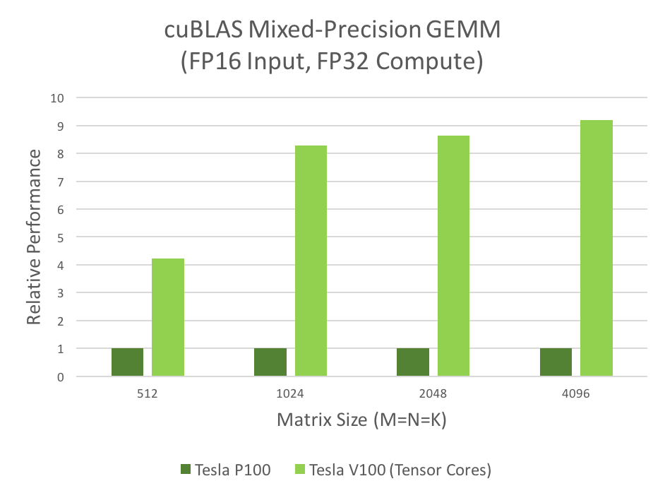
Many computational applications use GEMMs: signal processing, fluid dynamics, and many, many others. As the data sizes of these applications grow exponentially, these applications require matching increases in processing speed. The mixed-precision GEMM performance chart in figure 3 shows that Tensor Cores clearly answer this need.
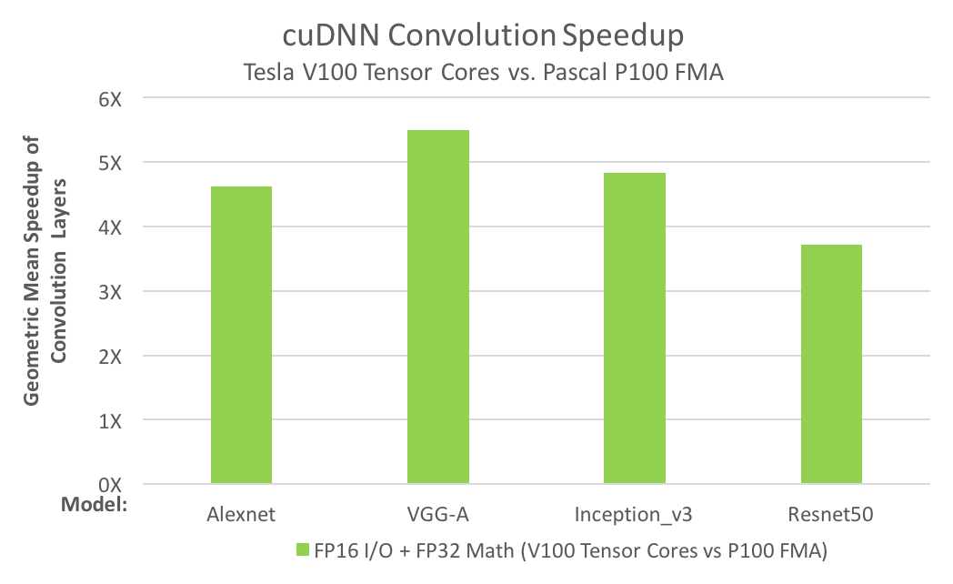
The need for convolution speed improvements is just as great; for example, today’s deep neural networks (DNNs) use many layers of convolutions. Artificial Intelligence researchers design deeper and deeper neural nets every year; the number of convolution layers in the deepest nets is now several dozen. Training DNNs requires the convolution layers to be run repeatedly, during both forward- and back-propagation. The convolution performance chart in Figure 4 shows that Tensor Cores answer the need for convolution performance. (You might also be interested in this recent post on effective techniques for mixed-precision neural network training)
Both performance charts show that Tesla V100’s Tensor Cores provide multiple times the performance of the previous-generation Tesla P100. Performance improvements this large change how work is done in computational fields: making interactivity possible, enabling “what-if” scenario studies, or reducing server farm usage. If you use GEMMs or convolutions in your applications, use the simple steps below to turbocharge your work.
How to Use Tensor Cores in cuBLAS
You can take advantage of Tensor Cores by making a few changes to your existing cuBLAS code. The changes are small changes in your use of the cuBLAS API.
The following sample code applies a few simple rules to indicate to cuBLAS that Tensor Cores should be used; these rules are enumerated explicitly after the code.
Sample code
The following code is largely the same as common code used to invoke a GEMM in cuBLAS on previous architectures.
// First, create a cuBLAS handle:
cublasStatus_t cublasStat = cublasCreate(&handle);

// Set the math mode to allow cuBLAS to use Tensor Cores:
cublasStat = cublasSetMathMode(handle, CUBLAS_TENSOR_OP_MATH);

// Allocate and initialize your matrices (only the A matrix is shown):
size_t matrixSizeA = (size_t)rowsA * colsA;
T_ELEM_IN **devPtrA = 0;

cudaMalloc((void**)&devPtrA[0], matrixSizeA * sizeof(devPtrA[0][0]));
T_ELEM_IN A  = (T_ELEM_IN *)malloc(matrixSizeA * sizeof(A[0]));

memset( A, 0xFF, matrixSizeA* sizeof(A[0]));
status1 = cublasSetMatrix(rowsA, colsA, sizeof(A[0]), A, rowsA, devPtrA[i], rowsA);

// ... allocate and initialize B and C matrices (not shown) ...

// Invoke the GEMM, ensuring k, lda, ldb, and ldc are all multiples of 8,
// and m is a multiple of 4:
cublasStat = cublasGemmEx(handle, transa, transb, m, n, k, alpha,
                          A, CUDA_R_16F, lda,
                          B, CUDA_R_16F, ldb,
                          beta, C, CUDA_R_16F, ldc, CUDA_R_32F, algo);
A Few Simple Rules
cuBLAS users will notice a few changes from their existing cuBLAS GEMM code:
- The routine must be a GEMM; currently, only GEMMs support Tensor Core execution.
- The math mode must be set to
CUBLAS_TENSOR_OP_MATH. Floating point math is not associative, so the results of the Tensor Core math routines are not quite bit-equivalent to the results of the analogous non-Tensor Core math routines. cuBLAS requires the user to “opt in” to the use of tensor cores. - All of
k,lda,ldb, andldcmust be a multiple of eight;mmust be a multiple of four. The Tensor Core math routines stride through input data in steps of eight values, so the dimensions of the matrices must be multiples of eight. - The input and output data types for the matrices must be either half precision or single precision. (Only
CUDA_R_16Fis shown above, butCUDA_R_32Falso is supported.)
GEMMs that do not satisfy the above rules will fall back to a non-Tensor Core implementation.
GEMM Performance
As mentioned, Tensor Cores deliver several times the GEMM performance over previous hardware. Figure 3 shows the comparative performance of GP100 (Pascal) to GV100 (Volta) hardware.
How to use Tensor Cores in cuDNN
Using Tensor Cores in cuDNN is also easy, and again involves only slight changes to existing code.
Sample Code
Sample code for using Tensor Cores in cuDNN can be found in conv_sample.cpp in the cuDNN samples directory; we have copied some excerpts below. (The cuDNN samples directory is packaged with the documentation.)
// Create a cuDNN handle:
checkCudnnErr(cudnnCreate(&handle_));

// Create your tensor descriptors:
checkCudnnErr( cudnnCreateTensorDescriptor( &cudnnIdesc ));
checkCudnnErr( cudnnCreateFilterDescriptor( &cudnnFdesc ));
checkCudnnErr( cudnnCreateTensorDescriptor( &cudnnOdesc ));
checkCudnnErr( cudnnCreateConvolutionDescriptor( &cudnnConvDesc ));

// Set tensor dimensions as multiples of eight (only the input tensor is shown here):
int dimA[] = {1, 8, 32, 32};
int strideA[] = {8192, 1024, 32, 1};

checkCudnnErr( cudnnSetTensorNdDescriptor(cudnnIdesc, getDataType(),
                                          convDim+2, dimA, strideA) );

// Allocate and initialize tensors (again, only the input tensor is shown):
checkCudaErr( cudaMalloc((void**)&(devPtrI), (insize) * sizeof(devPtrI[0]) ));
hostI = (T_ELEM*)calloc (insize, sizeof(hostI[0]) );

initImage(hostI, insize);

checkCudaErr( cudaMemcpy(devPtrI, hostI, sizeof(hostI[0]) * insize, cudaMemcpyHostToDevice));

// Set the compute data type (below as CUDNN_DATA_FLOAT):
checkCudnnErr( cudnnSetConvolutionNdDescriptor(cudnnConvDesc,
                                               convDim,
                                               padA,
                                               convstrideA,
                                               dilationA,
                                               CUDNN_CONVOLUTION,
                                               CUDNN_DATA_FLOAT) );

// Set the math type to allow cuDNN to use Tensor Cores:
checkCudnnErr( cudnnSetConvolutionMathType(cudnnConvDesc, CUDNN_TENSOR_OP_MATH) );

// Choose a supported algorithm:
cudnnConvolutionFwdAlgo_t algo = CUDNN_CONVOLUTION_FWD_ALGO_IMPLICIT_PRECOMP_GEMM;

// Allocate your workspace:
checkCudnnErr( cudnnGetConvolutionForwardWorkspaceSize(handle_, cudnnIdesc,
                                                       cudnnFdesc, cudnnConvDesc,
                                                       cudnnOdesc, algo, &workSpaceSize) );

if (workSpaceSize > 0) {
   cudaMalloc(&workSpace, workSpaceSize);
}

// Invoke the convolution:
checkCudnnErr( cudnnConvolutionForward(handle_, (void*)(&alpha), cudnnIdesc, devPtrI,
                                       cudnnFdesc, devPtrF, cudnnConvDesc, algo,
                                       workSpace, workSpaceSize, (void*)(&beta),
                                       cudnnOdesc, devPtrO) );
A Few Simple Rules
Notice a few changes from common cuDNN use:
- The convolution algorithm must be
ALGO_1(IMPLICIT_PRECOMP_GEMMfor forward). Other convolution algorithms besidesALGO_1may use Tensor Cores in future cuDNN releases. - The math type must be set to
CUDNN_TENSOR_OP_MATH. As in cuBLAS, the results of the Tensor Core math routines are not quite bit-equivalent to the results of the analogous non-tensor core math routines, so cuDNN requires the user to “opt in” to the use of Tensor Cores. - Both input and output channel dimensions must be a multiple of eight. Again as in cuBLAS, the Tensor Core math routines stride through input data in steps of eight values, so the dimensions of the input data must be multiples of eight.
- The input, filter, and output data types for the convolutions must be half precision.
Convolutions that do not satisfy the above rules will fall back to a non-Tensor Core implementation.
The above sample code shows NCHW data format, see the conv_sample.cpp sample for NHWC support as well.
Convolution Performance
As mentioned, Tensor Cores deliver several times the convolution performance over previous hardware. Figure 4 shows the comparative performance of GP100 (Pascal) to GV100 (Volta) hardware.
Programmatic Access to Tensor Cores in CUDA 9.0
Access to Tensor Cores in kernels via CUDA 9.0 is available as a preview feature. This means that the data structures, APIs and code described in this section are subject to change in future CUDA releases.
While cuBLAS and cuDNN cover many of the potential uses for Tensor Cores, you can also program them directly in CUDA C++. Tensor Cores are exposed in CUDA 9.0 via a set of functions and types in the nvcuda::wmma namespace. These allow you to load or initialize values into the special format required by the tensor cores, perform matrix multiply-accumulate (MMA) steps, and store values back out to memory. During program execution multiple Tensor Cores are used concurrently by a full warp. This allows the warp to perform a 16x16x16 MMA at very high throughput (Figure 5).

Let’s go through a simple example that shows how you can use the WMMA (Warp Matrix Multiply Accumulate) API to perform a matrix multiplication. Note that this example is not tuned for high performance and mostly serves as a demonstration of the API. For an example of optimizations you might apply to this code to get better performance, check out the cudaTensorCoreGemm sample in the CUDA Toolkit. For highest performance in production code cuBLAS should be used, as described above.
Headers and Namespaces
The WMMA API is contained within the mma.h header file. The complete namespace is nvcuda::wmma::*, but it’s useful to keep wmma explicit throughout the code, so we’ll just be using the nvcuda namespace.
#include <mma.h>
using namespace nvcuda;
Declarations and Initialization
The full GEMM specification allows the algorithm to work on transpositions of a or b, and for data strides to be larger than the strides in the matrix. For simplicity let’s assume that neither a nor b are transposed, and that the leading dimensions of the memory and the matrix are the same.
The strategy we’ll employ is to have a single warp responsible for a single 16×16 section of the output matrix. By using a two-dimensional grid and thread blocks, we can effectively tile the warps across the two dimensional output matrix.
// The only dimensions currently supported by WMMA
const int WMMA_M = 16;
const int WMMA_N = 16;
const int WMMA_K = 16;

__global__ void wmma_example(half *a, half *b, float *c,
                             int M, int N, int K,
                             float alpha, float beta)
{

    // Leading dimensions. Packed with no transpositions.
    int lda = M;
    int ldb = K;
    int ldc = M;

    // Tile using a 2D grid
    int warpM = (blockIdx.x * blockDim.x + threadIdx.x) / warpSize;
    int warpN = (blockIdx.y * blockDim.y + threadIdx.y);
Before the MMA operation is performed the operand matrices must be represented in the registers of the GPU. As an MMA is a warp-wide operation these registers are distributed amongst the threads of a warp with each thread holding a fragment of the overall matrix. The mapping between individual matrix parameters to their fragment(s) is opaque, so your program should not make assumptions about it.
In CUDA a fragment is a templated type with template parameters describing which matrix the fragment holds (A, B or accumulator), the shape of the overall WMMA operation, the data type and, for A and B matrices, whether the data is row or column major. This last argument can be used to perform transposition of either A or B matrices. This example does no transposition so both matrices are column major, which is standard for GEMM.
    // Declare the fragments
    wmma::fragment<wmma::matrix_a, WMMA_M, WMMA_N, WMMA_K, half, wmma::col_major> a_frag;
    wmma::fragment<wmma::matrix_b, WMMA_M, WMMA_N, WMMA_K, half, wmma::col_major> b_frag;
    wmma::fragment<wmma::accumulator, WMMA_M, WMMA_N, WMMA_K, float> acc_frag;
    wmma::fragment<wmma::accumulator, WMMA_M, WMMA_N, WMMA_K, float> c_frag;
The final part of the initialization step is to fill the accumulator fragment with zeros.
wmma::fill_fragment(acc_frag, 0.0f);
The Inner Loop
The strategy we’re using for the GEMM is to compute one tile of the output matrix per warp. To do this we need to loop over rows of the A matrix, and columns of the B matrix. This is along the K-dimension of both matrices and produces an MxN output tile. The load matrix function takes data from memory (global memory in this example, although it could be any memory space) and places it into a fragment. The third argument to the load is the “leading dimension” in memory of the matrix; the 16×16 tile we’re loading is discontinuous in memory so the function needs to know the stride between consecutive columns (or rows, if these were row-major fragments).
The MMA call accumulates in place, so both the first and last arguments are the accumulator fragment we previously initialized to zero.
    // Loop over the K-dimension
    for (int i = 0; i < K; i += WMMA_K) {
        int aRow = warpM * WMMA_M;
        int aCol = i;
        int bRow = i;
        int bCol = warpN * WMMA_N;

        // Bounds checking
        if (aRow < M && aCol < K && bRow < K && bCol < N) {
            // Load the inputs
            wmma::load_matrix_sync(a_frag, a + aRow + aCol * lda, lda);
            wmma::load_matrix_sync(b_frag, b + bRow + bCol * ldb, ldb);

            // Perform the matrix multiplication
            wmma::mma_sync(acc_frag, a_frag, b_frag, acc_frag);
        }
    }
Finishing Up
acc_frag now holds the result for this warp’s output tile based on the multiplication of A and B. The complete GEMM specification allows this result to be scaled, and for it to be accumulated on top of a matrix in place. One way to do this scaling is to perform element-wise operations on the fragment. Although the mapping from matrix coordinates to threads isn’t defined, element-wise operations do not need to know this mapping so can still be performed using fragments. As such, it’s legal to perform scaling operations on fragments or to add the contents of one fragment to another, so long as those two fragments have the same template parameters. If the fragments have different template parameters the results are undefined. Using this feature, we load in the existing data in C and, with the correct scaling, accumulate the result of the computation so far with it.
    // Load in current value of c, scale by beta, and add to result scaled by alpha
    int cRow = warpM * WMMA_M;
    int cCol = warpN * WMMA_N;

    if (cRow < M && cCol < N) {
        wmma::load_matrix_sync(c_frag, c + cRow + cCol * ldc, ldc, wmma::mem_col_major);

        for(int i=0; i < c_frag.num_elements; i++) {
            c_frag.x[i] = alpha * acc_frag.x[i] + beta * c_frag.x[i];
        }
Finally, we store the data out to memory. Once again the target pointer can be any memory space visible to the GPU and the leading dimension in memory must be specified. There is also an option to specify whether the output is to be written row or column major.
        // Store the output
        wmma::store_matrix_sync(c + cRow + cCol * ldc, c_frag, ldc, wmma::mem_col_major);
    }
}
With that, the matrix multiplication is complete. I’ve omitted the host code in this blog post, however a complete working example is available on Github.
Get Started with Tensor Cores in CUDA 9 Today
Hopefully this example has given you ideas about how you might use Tensor Cores in your application. If you’d like to know more, see the CUDA Programming Guide section on wmma.
The CUDA 9 Tensor Core API is a preview feature, so we’d love to hear your feedback. If you have any comments or questions please don’t hesitate to leave a comment below.
CUDA 9 is available free, so download it today.