 From Siri to Google Translate, deep neural networks have enabled breakthroughs in machine understanding of natural language. Most of these models treat language as a flat sequence of words or characters, and use a kind of model called a recurrent neural network (RNN) to process this sequence. But many linguists think that language is best understood as a hierarchical tree of phrases, so a significant amount of research has gone into deep learning models known as recursive neural networks that take this structure into account. While these models are notoriously hard to implement and inefficient to run, a brand new deep learning framework called PyTorch makes these and other complex natural language processing models a lot easier.
While recursive neural networks are a good demonstration of PyTorch’s flexibility, it is also a fully-featured framework for all kinds of deep learning with particularly strong support for computer vision. The work of developers at Facebook AI Research and several other labs, the framework combines the efficient and flexible GPU-accelerated backend libraries from Torch7 with an intuitive Python frontend that focuses on rapid prototyping, readable code, and support for the widest possible variety of deep learning models.
SPINNing Up
This post walks through the PyTorch implementation of a recursive neural network with a recurrent tracker and TreeLSTM nodes, also known as SPINN—an example of a deep learning model from natural language processing that is difficult to build in many popular frameworks. The implementation I describe is also partially batched, so it’s able to take advantage of GPU acceleration to run significantly faster than versions that don’t use batching.
This model, which stands for Stack-augmented Parser-Interpreter Neural Network, was introduced in Bowman et al. (2016) as a way of tackling the task of natural language inference using Stanford’s SNLI dataset.
The task is to classify pairs of sentences into three categories: assuming that sentence one is an accurate caption for an unseen image, then is sentence two (a) definitely, (b) possibly, or (c) definitely not also an accurate caption? (These classes are called entailment, neutral, and contradiction, respectively). For example, suppose sentence one is “two dogs are running through a field.” Then a sentence that would make the pair an entailment might be “there are animals outdoors,” one that would make the pair neutral might be “some puppies are running to catch a stick,” and one that would make it a contradiction could be “the pets are sitting on a couch.”
In particular, the goal of the research that led to SPINN was to do this by encoding each sentence into a fixed-length vector representation before determining their relationship (there are other ways, such as attentional models that compare individual parts of each sentence with each other using a kind of soft focus).
The dataset comes with machine-generated syntactic parse trees, which group the words in each sentence into phrases and clauses that all have independent meaning and are each composed of two words or sub-phrases. Many linguists believe that humans understand language by combining meanings in a hierarchical way as described by trees like these, so it might be worth trying to build a neural network that works the same way. Here’s an example of a sentence from the dataset, with its parse tree represented by nested parentheses:
( ( The church ) ( ( has ( cracks ( in ( the ceiling ) ) ) ) . ) )
One way to encode this sentence using a neural network that takes the parse tree into account would be to build a neural network layer Reduce that combines pairs of words (represented by word embeddings like GloVe) and/or phrases, then apply this layer recursively, taking the result of the last Reduce operation as the encoding of the sentence:
X = Reduce(“the”, “ceiling”)
Y = Reduce(“in”, X)
... etc.
But what if I want the network to work in an even more humanlike way, reading from left to right and maintaining sentence context while still combining phrases using the parse tree? Or, what if I want to train a network to construct its own parse tree as it reads the sentence, based on the words it sees? Here’s the same parse tree written a slightly different way:
The church ) has cracks in the ceiling ) ) ) ) . ) )
Or a third way, again equivalent:
WORDS:  The church   has cracks in the ceiling         .
PARSES: S   S      R S   S      S  S   S       R R R R S R R
All I did was remove open parentheses, then tag words with “S” for “shift” and replace close parentheses with “R” for “reduce.” But now the information can be read from left to right as a set of instructions for manipulating a stack and a stack-like buffer, with exactly the same results as the recursive method described above:
- Place the words into the buffer.
- Pop “The” from the front of the buffer and push it onto stack, followed by “church”.
- Pop top two stack values, apply Reduce, then push the result back to the stack.
- Pop “has” from buffer and push to stack, then “cracks”, then “in”, then “the”, then “ceiling”.
- Repeat four times: pop top two stack values, apply Reduce, then push the result.
- Pop “.” from buffer and push onto stack.
- Repeat two times: pop top two stack values, apply Reduce, then push the result.
- Pop the remaining stack value and return it as the sentence encoding.
I also want to maintain sentence context to take into account information about the parts of the sentence the system has already read when performing Reduce operations on later parts of the sentence. So I’ll replace the two-argument Reduce function with a three-argument function that takes a left child phrase, a right child phrase, and the current sentence context state. This state is created by a second neural network layer, a recurrent unit called the Tracker. The Tracker produces a new state at every step of the stack manipulation (i.e., after reading each word or close parenthesis) given the current sentence context state, the top entry b in the buffer, and the top two entries s1, s2 in the stack:
context[t+1] = Tracker(context[t], b, s1, s2)
You could easily imagine writing code to do these things in your favorite programming language. For each sentence to be processed it would load the next word from the buffer, run the Tracker, check whether to push onto the stack or perform a Reduce, do that operation, then repeat until the sentence is complete. Applied to a single sentence, this process constitutes a large and complex deep neural network with two trainable layers applied over and over in ways determined by the stack manipulation. But if you’re familiar with traditional deep learning frameworks like TensorFlow or Theano, it’s difficult to implement a dynamic procedure like this. It’s worth stepping back and spending a little while exploring why that’s the case, and what PyTorch does differently.
Graph Theory
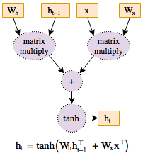
Deep neural networks are, in essence, just complicated functions with a large number of parameters. The goal of deep learning is to optimize these parameters by computing their partial derivatives (gradients) with respect to a loss metric. If the function is represented as a graph structure of computations (Figure 1), then traversing this graph backwards enables computing these gradients without any redundant work. Every modern framework for deep learning is based on this concept of backpropagation, and as a result every framework needs a way to represent computation graphs.
In many popular frameworks, including TensorFlow, Theano, and Keras, as well as Torch7’s nngraph library, the computation graph is a static object that is built ahead of time. The graph is defined using code that looks like mathematical expressions, but whose variables are actually placeholders that don’t yet hold any numerical values. This graph of placeholder variables is compiled once into a function that can then be run repeatedly on batches of training data to produce outputs and gradients.
This kind of static computation graph approach works well for convolutional networks, whose structure is typically fixed. But in many other applications, it would be useful if the graph structure of neural networks could vary depending on the data. In natural language processing, researchers usually want to unroll recurrent neural networks over as many timesteps as there are words in the input. The stack manipulation in the SPINN model described above relies heavily on control flow like for and if statements to define the graph structure of computation for a particular sentence. In even more complex cases, you might want to build models whose structure depends on the output of subnetworks within the model itself.
Some (though not all) of these ideas can be shoehorned into static-graph systems, but almost always at the cost of reduced transparency and confusing code. The framework has to add special nodes to its computation graphs that represent programming primitives like loops and conditionals, while users have to learn and use these nodes rather than the for and if statements in the language they’re writing their code in. This is because any control flow statements the programmer uses will run only once, when the graph is built, hard coding a single computation path.
For example, running a recurrent neural network unit (rnn_unit) over the vectors in words (starting with initial state h0) requires tf.while_loop, a special control flow node, in TensorFlow. An additional special node is needed to obtain the length of words at run time, since it’s only a placeholder at the time the code is run.
# TensorFlow
# (this code runs once, during model initialization)
# “words” is not a real list (it’s a placeholder variable) so
# I can’t use “len”
cond = lambda i, h: i < tf.shape(words)[0]
cell = lambda i, h: rnn_unit(words[i], h)
i = 0
_, h = tf.while_loop(cond, cell, (i, h0))
A fundamentally different approach, pioneered in decades of academic work including Harvard’s Kayak and autograd, as well as the research-centric frameworks Chainer and DyNet, is based on dynamic computation graphs. In such a framework, also known as define-by-run, the computation graph is built and rebuilt at runtime, with the same code that performs the computations for the forward pass also creating the data structure needed for backpropagation. This approach produces more straightforward code, because control flow can be written using standard for and if. It also makes debugging easier, because a run-time breakpoint or stack trace takes you to the code you actually wrote and not a compiled function in an execution engine. The same variable-length recurrent neural network can be implemented with a simple Python for loop in a dynamic framework.
# PyTorch (also works in Chainer)
# (this code runs on every forward pass of the model)
# “words” is a Python list with actual values in it
h = h0
for word in words:
    h = rnn_unit(word, h)
PyTorch is the first define-by-run deep learning framework that matches the capabilities and performance of static graph frameworks like TensorFlow, making it a good fit for everything from standard convolutional networks to the wildest reinforcement learning ideas. So let’s jump in and start looking at the SPINN implementation.
Code Review
Before I start building the network, I need to set up a data loader. It’s common in deep learning for models to operate on batches of data examples, to speed up training through parallelism and to have a smoother gradient at each step. I’d like to be able to do that here (I’ll explain later how the stack-manipulation process described above can be batched). The following Python code loads some data using a system built into the PyTorch text library that automatically produces batches by joining together examples of similar length. After running this code, train_iter, dev_iter, and test_iter contain iterators that cycle through batches in the train, validation, and test splits of SNLI.
from torchtext import data, datasets
TEXT = datasets.snli.ParsedTextField(lower=True)
TRANSITIONS = datasets.snli.ShiftReduceField()
LABELS = data.Field(sequential=False)
train, dev, test = datasets.SNLI.splits(
    TEXT, TRANSITIONS, LABELS, wv_type='glove.42B')
TEXT.build_vocab(train, dev, test)
train_iter, dev_iter, test_iter = data.BucketIterator.splits(
    (train, dev, test), batch_size=64)
You can find the rest of the code for setting up things like the training loop and accuracy metrics in train.py. Let’s move on to the model. As described above, a SPINN encoder contains a parameterized Reduce layer and an optional recurrent Tracker to keep track of sentence context by updating a hidden state every time the network reads a word or applies Reduce; the following code says that creating a SPINN just means creating these two submodules (we’ll see their code soon) and putting them in a container to be used later.
import torch
from torch import nn
# subclass the Module class from PyTorch’s neural network package
class SPINN(nn.Module):
    def __init__(self, config):
        super(SPINN, self).__init__()
        self.config = config
        self.reduce = Reduce(config.d_hidden, config.d_tracker)
        if config.d_tracker is not None:
            self.tracker = Tracker(config.d_hidden, config.d_tracker)
SPINN.__init__ is called once, when the model is created; it allocates and initializes parameters but doesn’t perform any neural network operations or build any kind of computation graph. The code that runs on each new batch of data is defined in the SPINN.forward method, the standard PyTorch name for the user-implemented method that defines a model’s forward pass. It’s effectively just an implementation of the stack-manipulation algorithm described above, in ordinary Python, operating on a batch of buffers and stacks—one of each for every example. I iterate over the set of “shift” and “reduce” operations contained in transitions, running the Tracker if it exists and going through each example in the batch to apply the “shift” operation if requested or add it to a list of examples that need the “reduce” operation. Then I run the Reduce layer on all the examples in that list and push the results back to their respective stacks.
def forward(self, buffers, transitions):
        # The input comes in as a single tensor of word embeddings;
        # I need it to be a list of stacks, one for each example in
        # the batch, that we can pop from independently. The words in
        # each example have already been reversed, so that they can
        # be read from left to right by popping from the end of each
        # list; they have also been prefixed with a null value.
        buffers = [list(torch.split(b.squeeze(1), 1, 0))
                   for b in torch.split(buffers, 1, 1)]
        # we also need two null values at the bottom of each stack,
        # so we can copy from the nulls in the input; these nulls
        # are all needed so that the tracker can run even if the
        # buffer or stack is empty
        stacks = [[buf[0], buf[0]] for buf in buffers]
        if hasattr(self, 'tracker'):
            self.tracker.reset_state()
        for trans_batch in transitions:
            if hasattr(self, 'tracker'):
                # I described the Tracker earlier as taking 4
                # arguments (context_t, b, s1, s2), but here I
                # provide the stack contents as a single argument
                # while storing the context inside the Tracker
                # object itself.
                tracker_states, _ = self.tracker(buffers, stacks)
            else:
                tracker_states = itertools.repeat(None)
            lefts, rights, trackings = [], [], []
            batch = zip(trans_batch, buffers, stacks, tracker_states)
            for transition, buf, stack, tracking in batch:
                if transition == SHIFT:
                    stack.append(buf.pop())
                elif transition == REDUCE:
                    rights.append(stack.pop())
                    lefts.append(stack.pop())
                    trackings.append(tracking)
            if rights:
                reduced = iter(self.reduce(lefts, rights, trackings))
                for transition, stack in zip(trans_batch, stacks):
                    if transition == REDUCE:
                        stack.append(next(reduced))
        return [stack.pop() for stack in stacks]
A call to self.tracker or self.reduce runs the forward method of the Tracker or Reduce submodule, respectively, which takes a list of examples on which to apply the operation. It makes sense to operate independently on the various examples here in the main forward method, keeping separate buffers and stacks for each of the examples in the batch, since all of the math-heavy, GPU-accelerated operations that benefit from batched execution take place in Tracker and Reduce. In order to write those functions more cleanly, I’ll use some helpers (which I’ll define later) which turn these lists of examples into batched tensors and vice versa.
I’d like the Reduce module to automatically batch its arguments to accelerate computation, then unbatch them so they can be independently pushed and popped later. The actual composition function used to combine the representations of each pair of left and right sub-phrases into the representation of the parent phrase is a TreeLSTM, a variation of the common recurrent neural network unit called an LSTM. This composition function requires that the state of each of the children actually consist of two tensors, a hidden state h and a memory cell state c, while the function is defined using two linear layers (nn.Linear) operating on the children’s hidden states and a nonlinear combination function tree_lstm that combines the result of the linear layers with the children’s memory cell states. In the SPINN, this is extended by adding a third linear layer that operates on the Tracker’s hidden state.
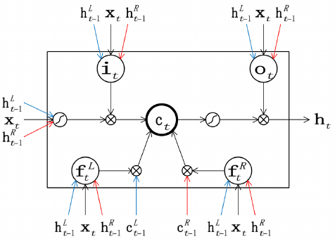
def tree_lstm(c1, c2, lstm_in):
    # Takes the memory cell states (c1, c2) of the two children, as
    # well as the sum of linear transformations of the children’s
    # hidden states (lstm_in)
    # That sum of transformed hidden states is broken up into a
    # candidate output a and four gates (i, f1, f2, and o).
    a, i, f1, f2, o = lstm_in.chunk(5, 1)
    c = a.tanh() * i.sigmoid() + f1.sigmoid() * c1 + f2.sigmoid() * c2
    h = o.sigmoid() * c.tanh()
    return h, c

class Reduce(nn.Module):
    def __init__(self, size, tracker_size=None):
        super(Reduce, self).__init__()
        self.left = nn.Linear(size, 5 * size)
        self.right = nn.Linear(size, 5 * size, bias=False)
        if tracker_size is not None:
            self.track = nn.Linear(tracker_size, 5 * size, bias=False)

    def forward(self, left_in, right_in, tracking=None):
        left, right = batch(left_in), batch(right_in)
        tracking = batch(tracking)
        lstm_in = self.left(left[0])
        lstm_in += self.right(right[0])
        if hasattr(self, 'track'):
            lstm_in += self.track(tracking[0])
        return unbatch(tree_lstm(left[1], right[1], lstm_in))
Since both the Reduce layer and the similarly implemented Tracker work using LSTMs, the batch and unbatch helper functions operate on pairs of hidden and memory states (h, c).
def batch(states):
    if states is None:
        return None
    states = tuple(states)
    if states[0] is None:
        return None
    # states is a list of B tensors of dimension (1, 2H)
    # this returns two tensors of dimension (B, H)
    return torch.cat(states, 0).chunk(2, 1)

def unbatch(state):
    if state is None:
        return itertools.repeat(None)
    # state is a pair of tensors of dimension (B, H)
    # this returns a list of B tensors of dimension (1, 2H)
    return torch.split(torch.cat(state, 1), 1, 0)
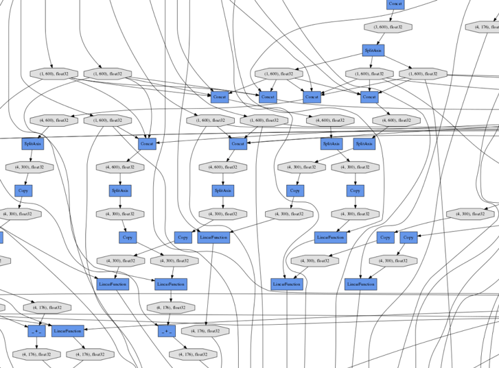
And that’s all there is to it. (The rest of the necessary code, including the Tracker, is in spinn.py, while the classifier layers that compute an SNLI category from two sentence encodings and compare this result with a target giving a final loss variable are in model.py). The forward code for SPINN and its submodules produces an extraordinarily complex computation graph (Figure 3) culminating in loss, whose details are completely different for every batch in the dataset, but which can be automatically backpropagated each time with very little overhead simply by calling loss.backward(), a function built into PyTorch that performs backpropagation from any point in a graph.
The models and hyperparameters in the full code can match the performance reported in the original SPINN paper, but are several times faster to train on a GPU because the implementation takes full advantage of batch processing and the efficiency of PyTorch. While the original implementation takes 21 minutes to compile the computation graph (meaning that the debugging cycle during implementation is at least that long), then about five days to train, the version described here has no compilation step and takes about 13 hours to train on a Tesla K40 GPU, or about 9 hours on a Quadro GP100.
Calling All Reinforcements
The version of the model described above without a Tracker is actually fairly well suited to TensorFlow’s new tf.fold domain-specific language for special cases of dynamic graphs, but the version with a Tracker would be much more difficult to implement. This is because adding a Tracker means switching from the recursive approach to the stack-based method. This (as in the code above) is most straightforwardly implemented using conditional branches that depend on the values of the input. But Fold lacks a built-in conditional branching operation, so the graph structure in a model built with it can depend only on the structure of the input and not its values. In addition, it would be effectively impossible to build a version of the SPINN whose Tracker decides how to parse the input sentence as it reads it since the graph structures in Fold—while they depend on the structure of an input example—must be completely fixed once an input example is loaded.
One such model was explored by researchers at DeepMind and Google Brain, who applied reinforcement learning to train a SPINN’s Tracker to parse input sentences without using any external parsing data. Essentially, such a model starts with random guessing and learns by rewarding itself when its parses happen to produce good accuracy on the overall classification task. The researchers wrote that they “use batch size 1 since the computation graph needs to be reconstructed for every example at every iteration depending on the samples from the policy network [Tracker]”—but PyTorch would enable them to use batched training even on a network like this one with complex, stochastically varying structure.
PyTorch is also the first framework to have reinforcement learning (RL) built into the library in the form of stochastic computation graphs, making policy gradient RL as easy to use as backpropagation. To add it to the model described above, you would simply need to rewrite the first few lines of the main SPINN for loop as follows, allowing the Tracker to define the probability of making each kind of parser transition.
!# nn.functional contains neural network operations without parameters
from torch.nn import functional as F
transitions = []
for i in range(len(buffers[0]) * 2 - 3):  # we know how many steps
    # obtain raw scores for each kind of parser transition
    tracker_states, transition_scores = self.tracker(buffers, stacks)
    # use a softmax function to normalize scores into probabilities,
    # then sample from the distribution these probabilities define
    transition_batch = F.softmax(transition_scores).multinomial()
    transitions.append(transition_batch
Then, once the batch has run all the way through and the model knows how accurately it predicted its categories, I can send reward signals back through these stochastic computation graph nodes in addition to backpropagating through the rest of the graph in the traditional way:
# losses should contain a loss per example, while mean and std
# represent averages across many batches
rewards = (-losses - mean) / std
for transition in transitions:
    transition.reinforce(rewards)
# connect the stochastic nodes to the final loss variable
# so that backpropagation can find them, multiplying by zero
# because this trick shouldn’t change the loss value
loss = losses.mean() + 0 * sum(transitions).sum()
# perform backpropagation through deterministic nodes and
# policy gradient RL for stochastic nodes
loss.backward()
The Google researchers reported results from SPINN plus RL that were a little bit better than what the original SPINN obtained on SNLI—despite the RL version using no precomputed parse tree information. The field of deep reinforcement learning for natural language processing is brand new, and research problems in the area are wide open; by building RL into the framework, PyTorch dramatically lowers the barrier to entry.
Learn More at GTC
Come to the GPU Technology Conference, May 8-11 in San Jose, California, to learn more about deep learning and PyTorch. GTC is the largest and most important event of the year for AI and GPU developers. Use code CMDLIPF to receive 20% off registration!
Join me at GTC and hear more about my work in my talk with Stephen Merity, Quasi-Recurrent Neural Networks – A Hightly Optimized RNN Architecture for the GPU (S7265). You’ll also enjoy Soumith Chintala’s talk, PyTorch, a Framework for New-Generation AI Research.
Get Started with PyTorch Today
Follow the instructions at pytorch.org to install on your chosen platform (Windows support is coming soon). PyTorch supports Python 2 and 3 and computation on either CPUs or NVIDIA GPUs using CUDA 7.5 or 8.0 and CUDNN 5.1 or 6.0. The Linux binaries for conda and pip even include CUDA itself, so you don’t need to set it up on your own.
The official tutorials include a 60-minute introduction and a walkthrough of Deep Q-Learning, a modern reinforcement learning model. There’s also a wonderfully comprehensive tutorial from Stanford’s Justin Johnson, while the official examples include—among other things—a deep convolutional generative adversarial network (DCGAN) and models for ImageNet and neural machine translation. Richie Ng from National University of Singapore keeps an up-to-date list of other PyTorch implementations, examples, and tutorials. The PyTorch developers and user community answer questions at all hours on the discussion forum, though you should probably check the API documentation first.
Even though PyTorch has only been available for a short time, three research papers have already used it several academic and industry labs have adopted it. Back when dynamic computation graphs were more obscure, my colleagues and I at Salesforce Research used to consider Chainer our secret sauce; now, we’re happy that PyTorch is bringing this level of power and flexibility into the mainstream, with the support of major companies. Happy hacking!


