TensorRT 3: Faster TensorFlow Inference and Volta Support

NVIDIA TensorRT™ is a high-performance deep learning inference optimizer and runtime that delivers low latency, high-throughput inference for deep learning applications. NVIDIA released TensorRT last year with the goal of accelerating deep learning inference for production deployment.

Figure 1. TensorRT optimizes trained neural network models to produce adeployment-ready runtime inference engine.

In this post we’ll introduce TensorRT 3, which improves performance versus previous versions and includes new features that make it easier to use. Key highlights of TensorRT 3 include:

TensorFlow Model Importer: a convenient API to import, optimize and generate inference runtime engines from TensorFlow trained models;
Python API: an easy to use use Python interface for improved productivity;
Volta Tensor Core Support: delivers up to 3.7x faster inference performance on Tesla V100 vs. Tesla P100 GPUs.

Let’s take a deep dive into the TensorRT workflow using a code example. We’ll cover importing trained models into TensorRT, optimizing them and generating runtime inference engines which can be serialized to disk for deployment. Finally, we’ll see how to load serialized runtime engines and run fast and efficient inference in production applications. But first, let’s go over some of the challenges of deploying inference and see why inference needs a dedicated solution.

Why Does Inference Need a Dedicated Solution?

As consumers of digital products and services, every day we interact with several AI powered services such as speech recognition, language translation, image recognition, and video caption generation, among others. Behind the scenes, a neural network computes the results for each query. This step is often called “inference”: new data is passed through a trained neural network to generate results. In traditional machine learning literature it’s also sometimes referred to as “prediction” or “scoring”.

This neural network usually runs within a web service in the cloud that takes in new requests from thousands or millions of users simultaneously, computes inference calculations for each request and serves the results back to users. To deliver a good user experience, all this has to happen under a small latency budget that includes network delay, neural network execution and other delays based on the production environment.

Similarly, if the AI application is running on a device such as in an autonomous vehicle performing real-time collision avoidance or a drone making real-time path planning decisions, latency becomes critical for vehicle safety. Power efficiency is equally important since these vehicles may have to go days, weeks or months between recharging or refueling.

Today, application developers and domain experts use GPU-accelerated deep learning frameworks such as Caffe, TensorFlow, or PyTorch to train deep neural networks to solve application-specific tasks. These frameworks give them the flexibility to prototype solutions by exploring network designs, performing model assessment and diagnostics and re-training models with new data.

Once the model is trained, developers typically follow one of the following deployment approaches.

Use a training framework such as Caffe, TensorFlow or others for production inference.
Build a custom deployment solution in-house using the GPU-accelerated cuDNN and cuBLAS libraries directly to minimize framework overhead.
Use training frameworks or build custom deployment solutions for CPU-only inference.

These deployment options often fail to deliver on key inference requirements such as scalability to millions of users, ability to process multiple inputs simultaneously, or ability to deliver results quickly and with high power efficiency.

More formally, the key requirements include:

High throughput: Deployed models have to process large volumes of data to serve a large number of users. Inefficient use of available resources leads to increased cloud or data center costs, and opportunity costs associated with serving fewer users.
Low response time: Applications such as speech recognition on mobile devices, and collision detection systems in cars demand results under a stringent low latency threshold. Inability to deliver results under these thresholds negatively affects the user experience of an app or may compromise driver safety in a car.
Power efficient: For deployment in data centers and low-power embedded devices power efficiency is critical. High power usage increases costs and may make embedded deployment solutions intractable.
Deployment-grade solution: Deployment environments require deployed software to be reliable and lightweight with minimal dependencies. Deep learning frameworks designed for model building, training and prototyping include additional packages and dependencies which introduce unnecessary overhead.

If you’re a developer of AI applications, you may relate to some or all of these challenges with deep learning deployment. NVIDIA TensorRT addresses these deployment challenges by optimizing trained neural networks to generate deployment-ready inference engines that maximize GPU inference performance and power efficiency. TensorRT runs with minimal dependencies on every GPU platform from datacenter GPUs such as P4 and V100, to autonomous driving and embedded platforms such as the Drive PX2 and Jetson TX2.

For more information on how TensorRT and NVIDIA GPUs deliver high-performance and efficient inference resulting in dramatic cost savings in the data center and power savings at the edge, refer to the following technical whitepaper: NVIDIA AI Inference Technical Overview.

Example: Deploying a TensorFlow model with TensorRT

While this post covers many of the basics of TensorRT for the sake of completeness, you can review the earlier post, Deploying Deep Neural Networks with NVIDIA TensorRT, for more details.

TensorRT 3 is faster, easier to use and introduces some new features that we’ll review as we go through the following code example. Jupyter (iPython) notebooks for this example are available on GitHub.

This simple example illustrates the steps necessary to import and optimize a trained TensorFlow neural network and deploy it as a TensorRT runtime engine. The example consists of two distinct steps:

Import and optimize trained models to generate inference engines
We perform this step only once, prior to deployment. We use TensorRT to parse a trained model and perform optimizations for specified parameters such as batch size, precision, and workspace memory for the target deployment GPU. The output of this step is an optimized inference execution engine which we serialize a file on disk called a plan file.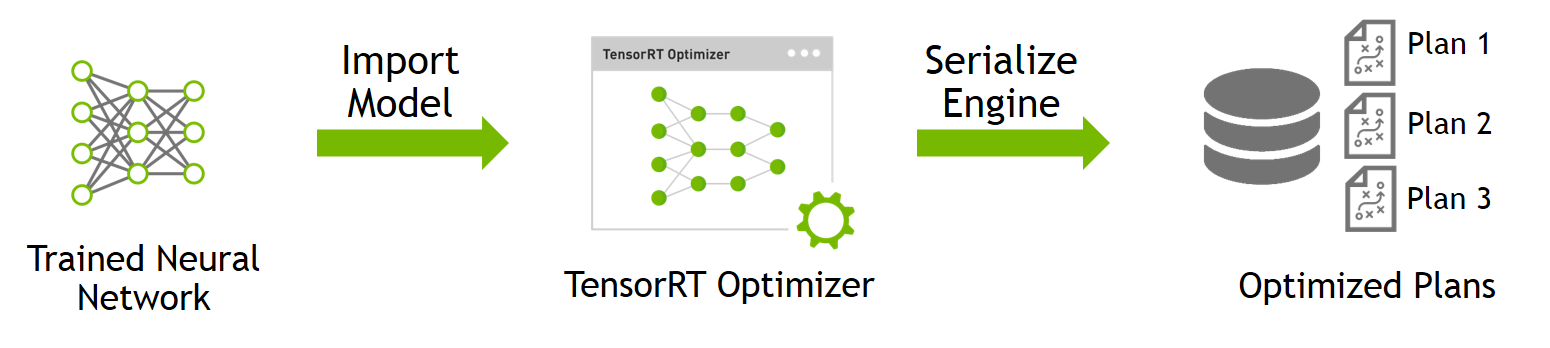
Deploy generated runtime inference engine for inference
This is the deployment step. We load and deserialize a saved plan file to create a TensorRT engine object, and use it to run inference on new data on the target deployment platform.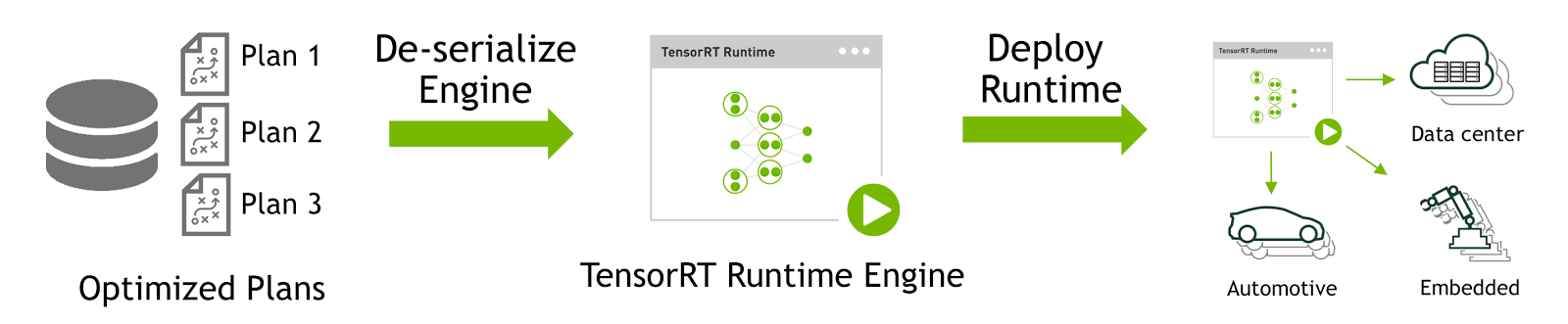

Importing a trained model

There are several deep learning frameworks, each with its own neural network structure definition and trained model file format. For Caffe and TensorFlow users, TensorRT provides simple and convenient Python and C++ APIs to import models for optimization.

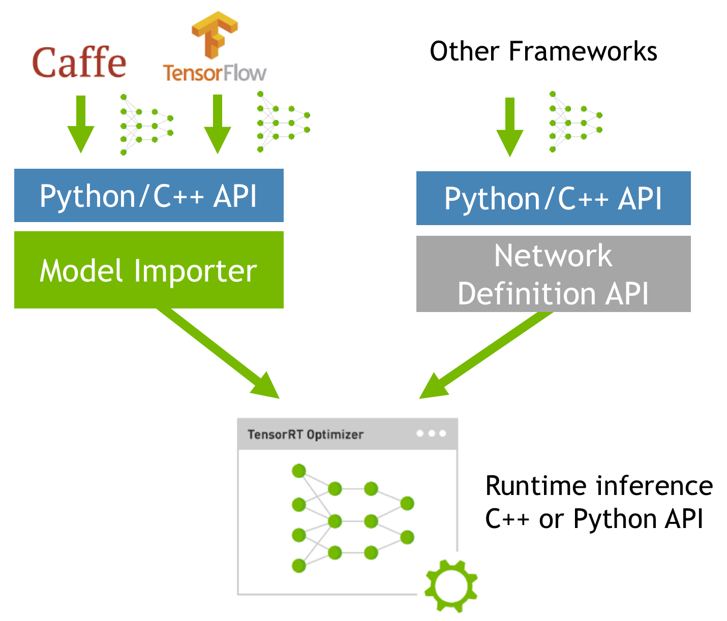
Figure 2. TensorRT provides model importers for Caffe and TensorFlow. Other framework models can be imported using the Network Definition API.

However, some open source and commercial frameworks, as well as proprietary in-house developed tools, have their own network definition formats. You can can use TensorRT’s Network Definition API to specify your network description (using either the C++ or the Python API) and load it into TensorRT to perform optimizations. Figure 2 shows the two different ways to get trained models into TensorRT.

Regardless of what approach you choose, once the model is imported, TensorRT performs the same set of model optimizations as illustrated in Figure 2.

We’ll start our example by importing necessary python packages and calling a function to import a TensorFlow model. Here we assume that you have TensorRT 3.0 installed and have a trained TensorFlow model that you’ve exported as a frozen model (.pb file) using the TensorFlow freeze_graph tool.

This example uses TensorRT 3’s Python API, but you can use the C++ API to do the same thing.

# Import TensorRT Modules
import tensorrt as trt
import uff
from tensorrt.parsers import uffparser
G_LOGGER = trt.infer.ConsoleLogger(trt.infer.LogSeverity.INFO)

# Load your newly created Tensorflow frozen model and convert it to UFF
uff_model = uff.from_tensorflow_frozen_model("keras_vgg19_frozen_graph.pb", ["dense_2/Softmax"])

UFF stands for Universal Framework Format, which is TensorRT’s internal format used to represent the network graph before running optimizations. The first argument to from_tensorflow_frozen_model() is the frozen trained model. In this example, we’re using a K eras VGG19 model. The second argument is the output layer name.

The output from the above step is a UFF graph representation of the TensorFlow model that is ready to be parsed by TensorRT. We configure the UFF parser below by providing the name and dimension (in CHW format) of the input layer and name of the output layer.

# Create a UFF parser to parse the UFF file created from your TF Frozen model
parser = uffparser.create_uff_parser()
parser.register_input("input_1", (3,224,224),0)
parser.register_output("dense_2/Softmax")

A Note on TensorRT Supported Layers

A lot of the innovation in neural network design these days centers around the invention of novel, custom layers. TensorRT supports the widely used standard layer types listed below. These should satisfy majority of neural network architectures:

Convolution
LSTM and GRU
Activation: ReLU, tanh, sigmoid
Pooling: max and average
Scaling
Element wise operations
LRN
Fully-connected
SoftMax
Deconvolution

However, deep learning is a rapidly evolving field and new layer types are introduced frequently. Many researchers and developers invent custom or proprietary layers specific to their applications. TensorRT provides a Custom Layer API to enable you to define your own custom layers that aren’t natively supported. These custom layers are defined using C++ to make it easy to leverage highly optimized CUDA libraries like cuDNN and cuBLAS. TensorRT will use your provided custom layer implementation when doing inference, as Figure 3 shows.

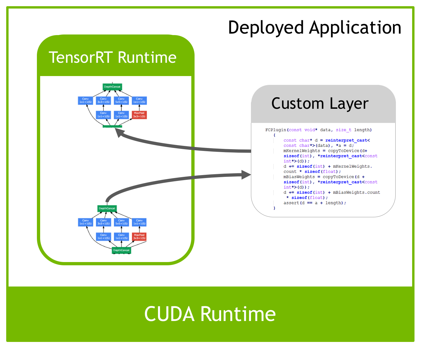
Figure 3. Custom layers can be integrated into the TensorRT runtime as plugins.

All layers in the VGG19 network in this example are supported by TensorRT, so we won’t demonstrate the process of writing a plugin. Refer to the TensorRT documentation for code samples and more details on writing custom layers.

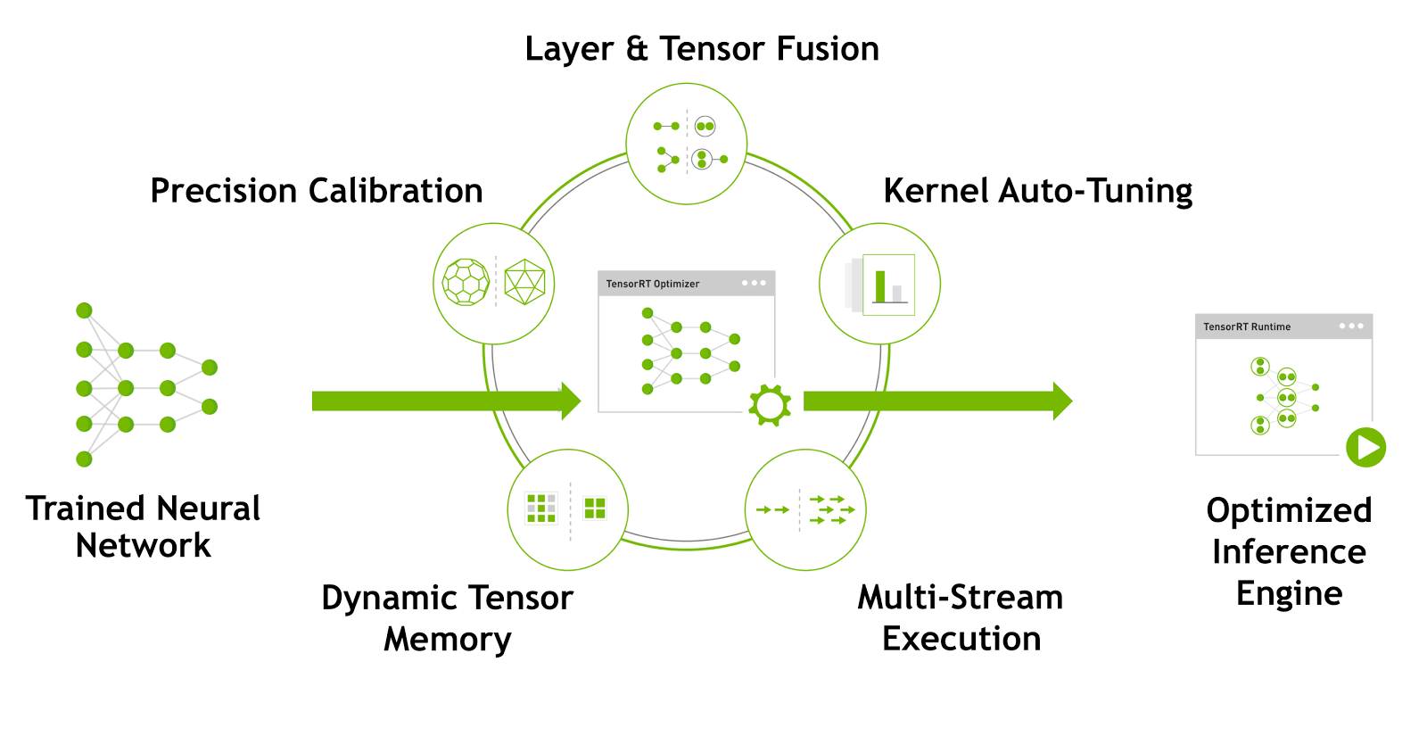
TensorRT Optimizations

Once you’ve imported the model into TensorRT, the next step is called the build phase, where you optimize the model for runtime execution. TensorRT can perform a number of optimizations, also illustrated in Figure 1:

Layer and tensor fusion and elimination of unused layers;
FP16 and INT8 reduced precision calibration;
Target-specific autotuning;
Efficient memory reuse

The build phase needs to be run on the target deployment GPU platform. For example, if your application is going to run on a Jetson TX2, the build needs to be performed on a Jetson TX2, and likewise if your inference services will run in the cloud on AWS P3 instances with Tesla V100 GPUs, then the build phase needs to run on a system with a Tesla V100.

This step is only performed once, so typical applications build one or many engines once, and then serialize them for later use.

TensorRT performs these optimizations automatically under the hood for you. All you need to specify is the UFF inference graph to optimize, the inference batch size, the amount of workspace GPU memory (used for CUDA kernel scratch space), and the target inference precision, as the following code shows.

# Build your TensorRT inference engine
# This step performs (1) Tensor fusion (2) Reduced precision 
# (3) Target autotuning (4) Tensor memory management
engine = trt.utils.uff_to_trt_engine(G_LOGGER, 
                                     uff_model,
                                     parser,
                                     1,
                                     1<<20, 
                                     trt.infer.DataType.FLOAT)

Here the uff_model is the one created from the Tensorflow frozen graph, the options specify FP32 inference with a batch size of 1 and 1MB of scratch space. The output of this step is an optimized runtime engine that is ready for inference.

Let’s take a closer look at what’s happening under the hood during the optimization step.

Optimization 1: Layer & Tensor Fusion

TensorRT parses the network computational graph and looks for opportunities to perform graph optimizations. These graph optimizations do not change the underlying computation in the graph: instead, they look to restructure the graph to perform the operations much faster and more efficiently.

For illustration, figure 4 shows a section of a neural network graph. Expert readers may recognize this as the “Inception” module from the GoogLeNet architecture which won the ImageNet competition in 2014.

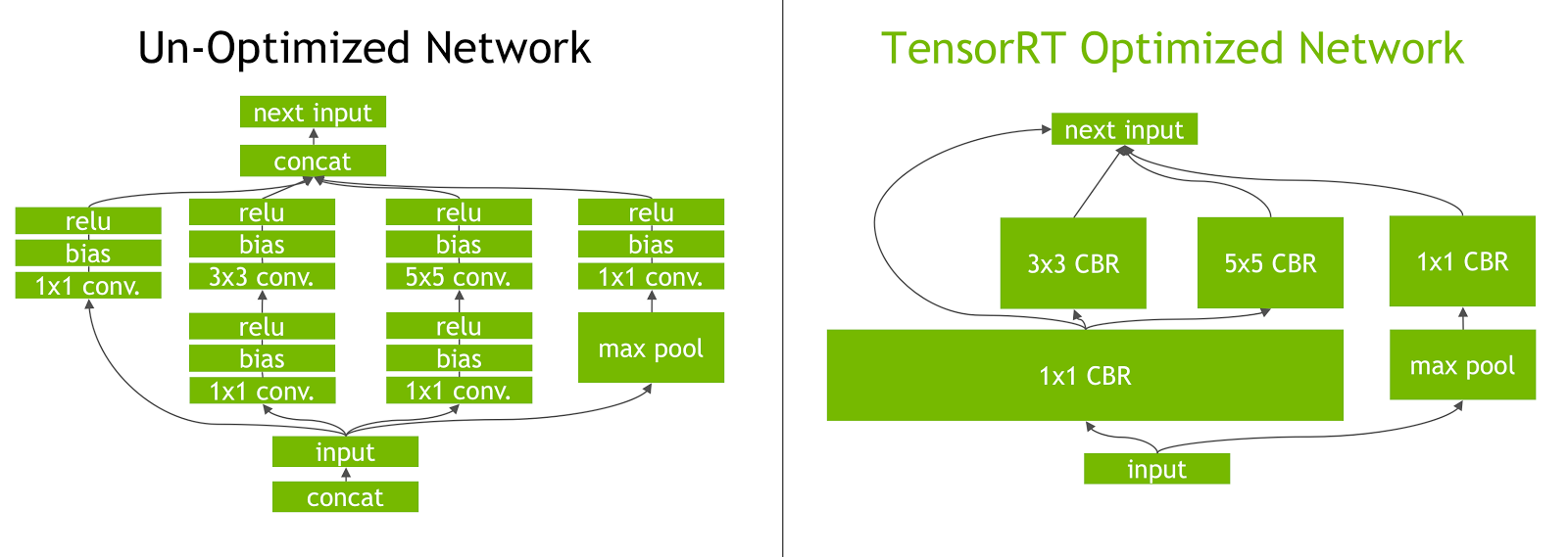
Figure 4. TensorRT’s vertical and horizontal layer fusion and layer elimination optimizations simplify the GoogLeNet Inception module graph, reducing computation and memory overhead.

When a deep learning framework executes this graph during inference, it makes multiple function calls for each layer. Since each operation is performed on the GPU, this translates to multiple CUDA kernel launches. The kernel computation is often very fast relative to the kernel launch overhead and the cost of reading and writing the tensor data for each layer. This results in a memory bandwidth bottleneck and underutilization of available GPU resources.

TensorRT addresses this by vertically fusing kernels to perform the sequential operations together. This layer fusion reduces kernel launches and avoids writing into and reading from memory between layers. In network on the left of Figure 4, the convolution, bias and ReLU layers of various sizes can be combined into a single kernel called CBR as the right side of Figure 4 shows. A simple analogy is making three separate trips to the supermarket to buy three items versus buying all three in a single trip.

TensorRT also recognizes layers that share the same input data and filter size, but have different weights. Instead of three separate kernels, TensorRT fuses them horizontally into a single wider kernel as shown for the 1×1 CBR layer in the right side of Figure 4.

TensorRT can also eliminate the concatenation layers in Figure 4 (“concat”) by preallocating output buffers and writing into them in a strided fashion.

Overall the result is a smaller, faster and more efficient graph with fewer layers and kernel launches, therefore reducing inference latency. Table 1 shows the results of TensorRT’s graph optimization for some common image classification networks.

Table 1: Number of layers before and after vertical and horizontal fusions and unused layer elimination.
Network	Layers	Layers after fusion
VGG19	43	27
Inception V3	309	113
ResNet-152	670	159

Optimization 2: FP16 and INT8 Precision Calibration

Most deep learning frameworks train neural networks in full 32-bit precision (FP32). Once the model is fully trained, inference computations can use half precision FP16 or even INT8 tensor operations, since gradient backpropagation is not required for inference. Using lower precision results in smaller model size, lower memory utilization and latency, and higher throughput.

TensorRT can deploy models in FP32, FP16 and INT8, and switching between them is as easy as specifying the data type in the uff_to_trt_engine function:

For FP32, use trt.infer.DataType.FLOAT.
For FP16 in and FP16 Tensor Cores on Volta GPUs, use trt.infer.DataType.HALF
For INT8 inference, use trt.infer.DataType.INT8.

You can see in Table 2 that the dynamic range of INT8 is dramatically smaller than full-precision dynamic range. INT8 can only represent 256 different values. To quantize full-precision information into INT8 while minimizing accuracy loss, TensorRT must perform a process called calibration to determine how best to represent the weights and activations as 8-bit integers.

The calibration step requires you to provide TensorRT with a representative sample of the input training data. No additional fine tuning or retraining of the model is necessary, and you don’t need to have access to the entire training dataset. Calibration is a completely automated and parameter-free method for converting FP32 to INT8.

In this example, we’re only demonstrating FP32 and FP16 deployment, please refer to the TensorRT documentation for code samples and more details on how to perform the calibration step.

Table 2: INT8 has significantly lower dynamic range and precision compared to FP32. TensorRT quantizes weights and activations from FP32 to INT8 using a calibration process that minimizes information loss.
Precision	Dynamic Range
FP32	-3.4×10³⁸ ~ +3.4×10³⁸
FP16	-65504 ~ +65504
INT8	-128 ~ +127

Optimization 3: Kernel Auto-Tuning

During the optimization phase TensorRT also chooses from hundreds of specialized kernels, many of them hand-tuned and optimized for a range of parameters and target platforms. As an example, there are several different algorithms to do convolutions. TensorRT will pick the implementation from a library of kernels that delivers the best performance for the target GPU, input data size, filter size, tensor layout, batch size and other parameters.

This ensures that the deployed model is performance tuned for the specific deployment platform as well as for the specific neural network being deployed.

Optimization 4: Dynamic Tensor Memory

TensorRT also reduces memory footprint and improves memory reuse by designating memory for each tensor only for the duration of its usage, avoiding memory allocation overhead for fast and efficient execution.

TensorRT Optimization Performance Results

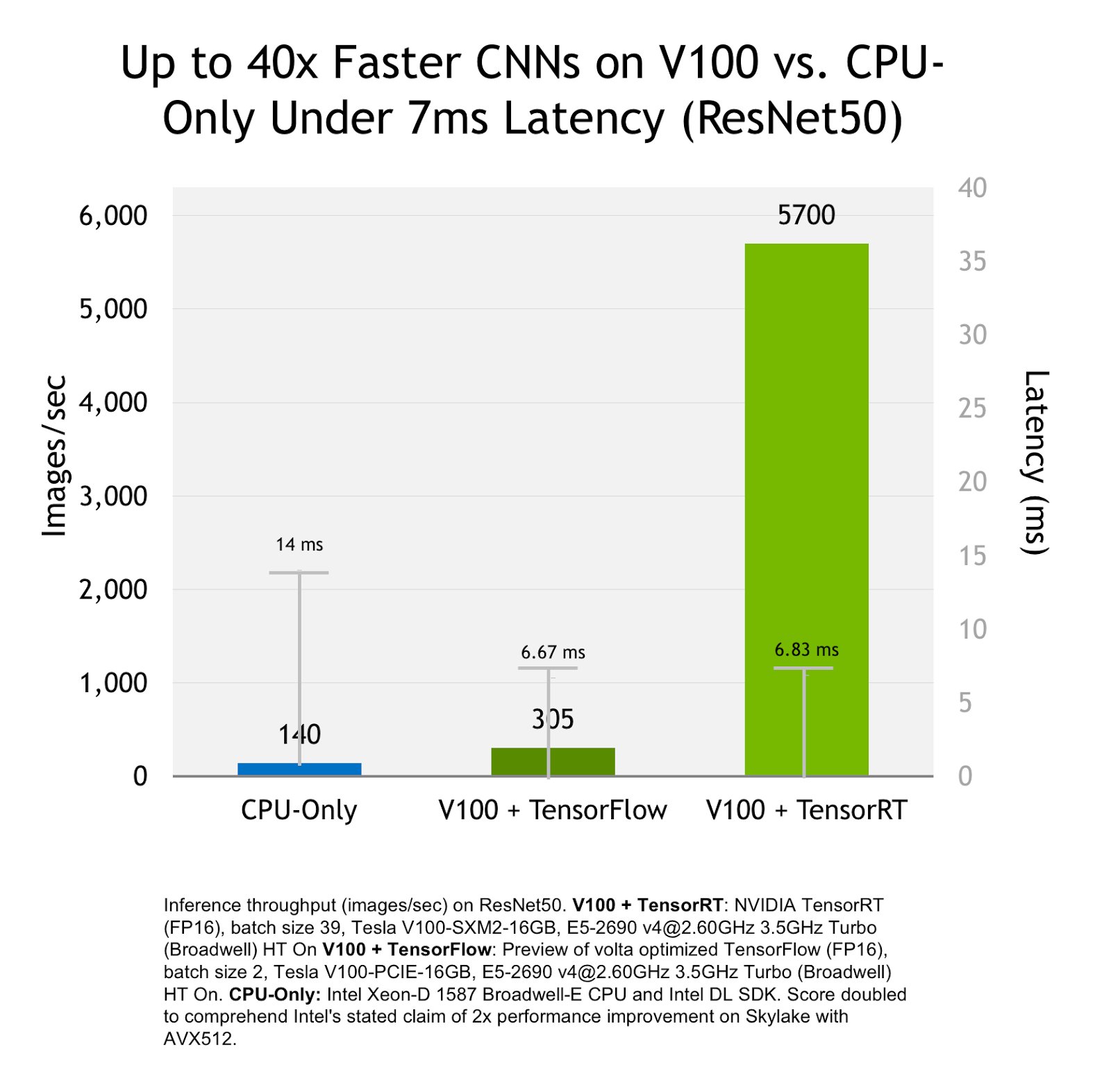
The result of all of TensorRT’s optimizations is that models run faster and more efficiently compared to running inference using deep learning frameworks on CPU or GPU. The chart in Figure 5 compares inference performance in images/sec of the ResNet-50 network on a CPU, on a Tesla V100 GPU with TensorFlow inference and on a Tesla V100 GPU with TensorRT inference.

With TensorRT, you can get up to 40x faster inference performance comparing Tesla V100 to CPU. TensorRT inference with TensorFlow models running on a Volta GPU is up to 18x faster under a 7ms real-time latency requirement.

Figure 5. TensorRT inference performance compared to CPU-only inference and TensorFlow framework inference.

Serializing Optimized TensorRT Engines

The output of the TensorRT optimization phase is is a runtime inference engine that can be serialized to disk. This serialized file is called a “plan” file that includes serialized data that the runtime engine uses to execute the network. It’s called a plan file because it includes not only the weights, but also the schedule for the kernels to execute the network. It also includes information about the network that the application can query in order to determine how to bind input and output buffers.

Use TensorRT’s write_engine_to_file() function to perform the serialization.

# Serialize TensorRT engine to a file for when you are ready to deploy your model.
trt.utils.write_engine_to_file("keras_vgg19_b1_FP32.engine", 
                               engine.serialize())

TensorRT Run-Time Inference

You’re now ready to deploy your application with TensorRT. To quickly recap, you’ve so far imported a trained TensorFlow model into TensorRT, and performed a number of optimizations to generate a runtime engine. And you’ve serialized this engine to disk as an engine plan file. You performed all these steps offline, and only once prior to deployment.

The next step is to load serialized models into your runtime environment and perform inference on new data. To demonstrate this step, we’ll use the TensorRT Lite API. This is a highly abstracted interface that handles a lot of the standard tasks like creating the logger, deserializing the engine from a plan file to create a runtime, and allocating GPU memory for the engine. During inference, it also manages data transfer to and from GPU automatically, so you can just create an engine and start processing data. For more fine-grained control, you can always use the standard API or the C++ API.

from tensorrt.lite import Engine
from tensorrt.infer import LogSeverity
import tensorrt

# Create a runtime engine from plan file using TensorRT Lite API 
engine_single = Engine(PLAN="keras_vgg19_b1_FP32.engine",
                       postprocessors={"dense_2/Softmax":analyze})

images_trt, images_tf = load_and_preprocess_images()

results = []
for image in images_trt:
    result = engine_single.infer(image) # Single function for inference
    results.append(result)

Conclusion

TensorRT addresses three key challenges for deep learning deployment.

High throughput and low latency: TensorRT performs layer fusion, precision calibration, and target auto-tuning to deliver up to 40x faster inference vs. CPU and up to 18x faster inference of TensorFlow models on Volta GPUs under 7ms real time latency, as Figure 5 shows. This means you can easily scale your AI application to serve more users due to better utilization of GPU resources.
Power-efficiency: With target-specific optimizations and dynamic memory management, TensorRT delivers higher power efficiency compared to deep learning framework inference. Low-power devices run longer and data centers run cooler.
Deployment-grade solution: TensorRT is designed for deployment. With TensorRT you deploy a lightweight runtime without framework dependencies and overhead. With its Python and C++ interfaces, TensorRT is easy to use for everyone from researchers and data scientists training models, to developers building production deployment applications.

TensorRT 3 is now available as a free download to all members of the NVIDIA developer program. Please visit the TensorRT home page to learn more and download TensorRT today!

TensorRT is also available as a container on NVIDIA GPU CLOUD for use on-premises or on AWS P3 instances. Sign up for an NGC account to get free access to the TensorRT container as well as NVIDIA optimized deep learning framework containers for training.

We hope you enjoyed reading this post. If you have questions, comments or feedback please use the comments section below. You can also file a bug or feature request from your NVIDIA developer account by navigating to the account page > My Bugs > Submit a New Bug. We look forward to your feedback.