 This post is an excerpt from Chapter 4 of the book CUDA Fortran for Scientists and Engineers, by Gregory Ruetsch and Massimiliano Fatica. In this excerpt we extend the matrix transpose example from a previous post to operate on a matrix that is distributed across multiple GPUs. The data layout is shown in Figure 1 for an
 nx × ny = 1024 × 768 element matrix that is distributed amongst four devices. Each device contains a horizontal slice of the input matrix shown in the figure, as well as a horizontal slice of the output matrix. These input matrix slices of 1024 × 192 elements are divided into four tiles containing 256 × 192 elements each, which are referred to as p2pTile in the code. As the name indicates, the p2pTiles are used for peer-to-peer transfers. After a p2pTile has been transferred to the appropriate device if necessary (tiles on the block diagonal do not need to be transferred as the input and output tiles are on the same device), a CUDA transpose kernel launch transposes the elements within the p2pTile using thread blocks that process smaller tiles of 32 × 32 elements.
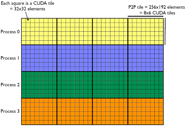
MARKDOWN_HASH97893f46e7e13ef37b4c2e0ac60d85caMARKDOWN_HASH x MARKDOWN_HASH531beb50ffb32d08756e6462c037c8e1MARKDOWN_HASH = 1024 x 768 matrix on four devices. Each device holds a 1024 x 192 horizontal slice of input matrix (as well as a 768 x 256 horizontal slice of the output matrix). Each slice of the input matrix is broken into four tiles of 256 x 192 elements, which are used for peer-to-peer transfers. The CUDA kernel transposes this tile using 48 thread blocks, each of which processes a 32 x 32 tile.The full code is available on the website for the CUDA Fortran for Scientists and Engineers textbook [line numbers below refer to the file CUDAFortranCode/chapter4/P2P/transposeP2P.cuf in the source code archive]. In this post we pull in only the relevant parts for our discussion. We start the discussion of the code with the transpose kernel:
  attributes(global) subroutine cudaTranspose( &
       odata, ldo, idata, ldi)
    implicit none
    real, intent(out) :: odata(ldo,*)
    real, intent(in) :: idata(ldi,*)
    integer, value, intent(in) :: ldo, ldi
    real, shared :: tile(cudaTileDim+1, cudaTileDim)
    integer :: x, y, j

    x = (blockIdx%x-1) * cudaTileDim + threadIdx%x
    y = (blockIdx%y-1) * cudaTileDim + threadIdx%y

    do j = 0, cudaTileDim-1, blockRows
       tile(threadIdx%x, threadIdx%y+j) = idata(x,y+j)
    end do

    call syncthreads()

    x = (blockIdx%y-1) * cudaTileDim + threadIdx%x
    y = (blockIdx%x-1) * cudaTileDim + threadIdx%y

    do j = 0, cudaTileDim-1, blockRows
       odata(x,y+j) = tile(threadIdx%y+j, threadIdx%x)
    end do
  end subroutine cudaTranspose
This transpose is basically the same kernel we developed in our previous post for the single-GPU transpose, with the exception that two additional parameters are passed to the kernel, ldi and ldo, the leading dimensions of the input and output matrices. These parameters are needed because each kernel call transposes a submatrix of each device’s slice of the matrix. One could do without modifying the kernel at all by copying data to and from a temporary array, but such intermediate data transfers would greatly affect performance. Note that the leading dimension parameters are only used in the declaration of the input and output matrices on lines 17 and 18—the rest of the code is identical to the single-GPU code. Most of the host code performs mundane tasks such as getting the number and types of devices (lines 85-94), checking that all devices are peer-to-peer capable and enabling peer-to-peer communication (lines 96-119), verifying that the matrix divides evenly into the various tile sizes (121-140), printing out the various sizes (lines 146-165), and initializing host data and transposing on the host (lines 169-170). Because we want to overlap the execution of the transpose kernel with the data transfer between GPUs, we want to avoid using the default stream for peer-to-peer communication as well as kernel execution. We want each device to have nDevicesnDevices devices, each requiring nDevices streams, we use a two dimensional variable to hold the stream IDs:
allocate(streamID(0:nDevices-1,0:nDevices-1))
  do p = 0, nDevices-1
     istat = cudaSetDevice(p)
     do stage = 0, nDevices-1
        istat = cudaStreamCreate(streamID(p,stage))
     enddo
  enddo
where the first index to streamID corresponds to the particular device the stream is associated with, and the second index refers to the stages of the calculation. The stages of the transpose, enumerated zero to nDevices-1, are organized as follows. In the zeroth stage, each device transposes the submatrix that lies along the block diagonal of the global matrix, which is depicted in the top diagram of Figure 2. This is done first as no peer-to-peer communication is involved, and the kernel execution can overlap data transfers in the first stage.
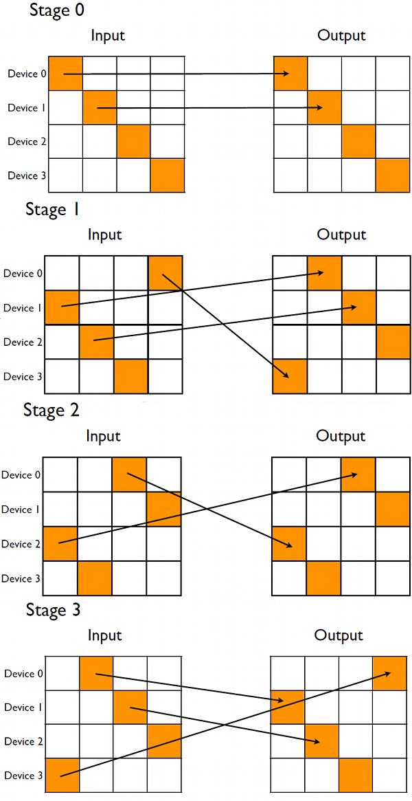
In stage one, data from what is primarily the first block-subdiagonal of the input matrix is sent to the devices which hold the corresponding first block-superdiagonal, as depicted in Figure 2. After the transfer completes, the receiving device performs the transpose. Note that one of the blocks transferred during stage one is not on the subdiagonal, as we wrap the pattern so that all devices both send and receive data during each stage. The following stages do similar operations on additional block sub- and super-diagonals until all of the blocks have been transposed. The wrapping during these stages becomes more pronounced, so that in the final stage the communication pattern is the reverse of the first stage. In using this arrangement, during each stage other than the zeroth, each device sends and receives a block of data, and both of these transfers can overlap if transferred asynchronously since the devices have separate send and receive copy engines. The distributed global matrices are stored using the derived type deviceArray:
! distributed arrays
  type deviceArray
     real, device, allocatable :: v(:,:)
  end type deviceArray

  type (deviceArray), allocatable :: &
       d_idata(:), d_tdata(:), d_rdata(:)  ! (0:nDevices-1)
This same technique was used in the p2pBandwidth code in Chapter 4 of CUDA Fortran for Scientists and Engineers. Instances of this derived type will be host data, but the member v is device data. There are three allocatable array declarations of this derived type on line 74: d_idata for the input data, d_rdata which is a receive buffer used in the transfers, and d_tdata which holds the final transposed data. These variables are allocated by:
  allocate(d_idata(0:nDevices-1),&
       d_tdata(0:nDevices-1), d_rdata(0:nDevices-1))
which represents decomposition of the global array into the horizontal slices depicted in Figure 2. The members of the derived type hold the horizontal slices, which are allocated and initialized by:
  do p = 0, nDevices-1
     istat = cudaSetDevice(p)
     allocate(d_idata(p)%v(nx,p2pTileDimY), &
          d_rdata(p)%v(nx,p2pTileDimY), &
          d_tdata(p)%v(ny,p2pTileDimX))

     yOffset = p*p2pTileDimY
     d_idata(p)%v(:,:) = h_idata(:, &
          yOffset+1:yOffset+p2pTileDimY)
     d_rdata(p)%v(:,:) = -1.0
     d_tdata(p)%v(:,:) = -1.0
  enddo
where nx and ny are the global matrix sizes, and p2pTileDimY and p2pTileDimX are the sizes of the horizontal slices of the input and transposed matrices, respectively. Note that the device is set on line 194 to the appropriate device before each member v is allocated. Also, since the matrix on the host is stored in h_idata(nx,ny), the offset yOffset is used when initializing d_idata on lines 200-201. The code which performs the various transpose stages is:
  ! Stage 0:
  ! transpose diagonal blocks (local data) before kicking off
  ! transfers and transposes of other blocks

  do p = 0, nDevices-1
     istat = cudaSetDevice(p)
     if (asyncVersion) then
        call cudaTranspose &
             <<<dimgrid, dimblock,="" 0,="" streamid(p,0)="">>> &
             (d_tdata(p)%v(p*p2pTileDimY+1,1), ny, &
             d_idata(p)%v(p*p2pTileDimX+1,1), nx)
     else
        call cudaTranspose<<<dimgrid, dimblock="">>> &
             (d_tdata(p)%v(p*p2pTileDimY+1,1), ny, &
             d_idata(p)%v(p*p2pTileDimX+1,1), nx)
     endif
  enddo

  ! now send data to blocks to the right of diagonal
  ! (using mod for wrapping) and transpose

  do stage = 1, nDevices-1    ! stages = offset diagonals
     do rDev = 0, nDevices-1  ! device that receives
        sDev = mod(stage+rDev, nDevices)  ! dev that sends

        if (asyncVersion) then
           istat = cudaSetDevice(rDev)
           istat = cudaMemcpy2DAsync( &
                d_rdata(rDev)%v(sDev*p2pTileDimX+1,1), nx, &
                d_idata(sDev)%v(rDev*p2pTileDimX+1,1), nx, &
                p2pTileDimX, p2pTileDimY, &
                stream=streamID(rDev,stage))
        else
           istat = cudaMemcpy2D( &
                d_rdata(rDev)%v(sDev*p2pTileDimX+1,1), nx, &
                d_idata(sDev)%v(rDev*p2pTileDimX+1,1), nx, &
                p2pTileDimX, p2pTileDimY)
        end if

        istat = cudaSetDevice(rDev)
        if (asyncVersion) then
           call cudaTranspose &
                <<<dimgrid, dimblock,="" 0,="" &="" streamid(rdev,stage)="">>>  &
                (d_tdata(rDev)%v(sDev*p2pTileDimY+1,1), ny, &
                d_rdata(rDev)%v(sDev*p2pTileDimX+1,1), nx)
        else
           call cudaTranspose<<<dimgrid, dimblock="">>> &
                (d_tdata(rDev)%v(sDev*p2pTileDimY+1,1), ny, &
                d_rdata(rDev)%v(sDev*p2pTileDimX+1,1), nx)
        endif
     enddo
  enddo
Stage 0 occurs in the loop on lines 220-232. After the device is set on line 221, the transpose of the diagonal block is performed either using the default, blocking stream on line 228, or in a non-default stream on line 223. The parameter asyncVersion is used to toggle between asynchronous and synchronous execution. The execution configuration used in the kernel launches is determined by:
  dimGrid = dim3(p2pTileDimX/cudaTileDim, &
       p2pTileDimY/cudaTileDim, 1)
  dimBlock = dim3(cudaTileDim, blockRows, 1)
where the thread block is the same as in the single-GPU case, and each kernel launch operates on a submatrix of size p2pTileDimX × p2pTileDimY. The other stages are performed in the loop from line 237-268. After the sending and receiving devices are determined on lines 238 and 239, the peer-to-peer transfer is performed using either cudaMemcpy2DAsync() or cudaMemcpy2D(), depending on asyncVersion. If the asynchronous version is used, then the device is set to the receiving device on line 242, and accordingly the non-default stream used for the transfer is the stream associated with the receiving device. We use the stream associated with the device receiving the data rather than the device sending the data because we want to block the launch of the transpose kernel on the receiving device until the transfer is complete. This is accomplished by default when the same stream is used for the transfer and transpose. For the synchronous data transfer, the device does not need to be specified via cudaSetDevice(). Note that the array receiving the data is in d_rdata. The out-of-place transpose from d_rdata to d_tdata is then performed by the kernel launch on line 257 or 263. Regardless of whether the default stream is used or not, the device must be set as done on line 255. The remainder of the code transfers the data back to the host, checks for correctness, and reports the effective bandwidth. Timing in this case is done using a wall-clock timer. This code uses the C function gettimeofday():
#include
#include <sys/types.h>
#include
#include

double wallclock()
{
  struct timeval tv;
  struct timezone tz;
  double t;

  gettimeofday(&tv, &tz);

  t = (double)tv.tv_sec;
  t += ((double)tv.tv_usec)/1000000.0;

  return t;
}
which is accessed in the Fortran code using the {\tt timing} module:
module timing
  interface wallclock
     function wallclock() result(res) bind(C, name='wallclock')
       use iso_c_binding
       real (c_double) :: res
     end function wallclock
  end interface wallclock
end module timing
Whenever this routine is called, we explicitly check to make sure there is no pending or executing operations on the device:
  ! wait for execution to complete and get wallclock
  do p = 0, nDevices-1
     istat = cudaSetDevice(p)
     istat = cudaDeviceSynchronize()
  enddo
  timeStop = wallclock()
Note that most of this multi-GPU code is overhead associated with declaring and initializing arrays and enabling peer-to-peer communication. The actual data transfers and kernel launches are contained in approximately 50 lines of code, which contains branches for synchronous and asynchronous execution. The transpose kernel itself is only slightly modified from the single-GPU transpose to allow for arbitrary leading dimensions of the arrays. We use a compute node with two devices for running this transpose code. To compare to the single-GPU transpose results, which used 1024 × 1024 matrices, we choose an overall matrix size of 2048 × 2048. In this case each transpose kernel processes a 1024 × 1024 submatrix, the same as in the single-GPU case. When using blocking transfers we obtain the results:
Number of CUDA-capable devices: 2

  Device 0: Tesla M2050
  Device 1: Tesla M2050

Array size: 2048x2048

CUDA block size: 32x8,  CUDA tile size: 32x32
dimGrid: 32x32x1,   dimBlock: 32x8x1

nDevices: 2,  Local input array size: 2048x1024
p2pTileDim: 1024x1024

async mode:  F

Bandwidth (GB/s):   16.43
and when using asynchronous transfers we have:
Number of CUDA-capable devices: 2

  Device 0: Tesla M2050
  Device 1: Tesla M2050

Array size: 2048x2048

CUDA block size: 32x8,  CUDA tile size: 32x32
dimGrid: 32x32x1,   dimBlock: 32x8x1

nDevices: 2,  Local input array size: 2048x1024
p2pTileDim: 1024x1024

async mode:  T

Bandwidth (GB/s):   29.73
While both these numbers fall short of the effective bandwidth achieved in the single-GPU case, one must take into account that half of the data is being transferred over the PCIe bus, which is over an order of magnitude slower than the global memory bandwidth within a GPU. In light of this the use of asynchronous transfers which overlap kernel execution is very advantageous as can be seen from the results. In addition, typically the transpose is used as a means to some other operation that can be done in parallel, in which case cost of the PCI transfer is further amortized. If you enjoyed this post, please check out the book CUDA Fortran for Scientists and Engineers, as well as the related posts linked below.