In part 1 of this series I introduced Generative Adversarial Networks (GANs) and showed how to generate images of handwritten digits using a GAN. In this post I will do something much more exciting: use Generative Adversarial Networks to generate images of celebrity faces.
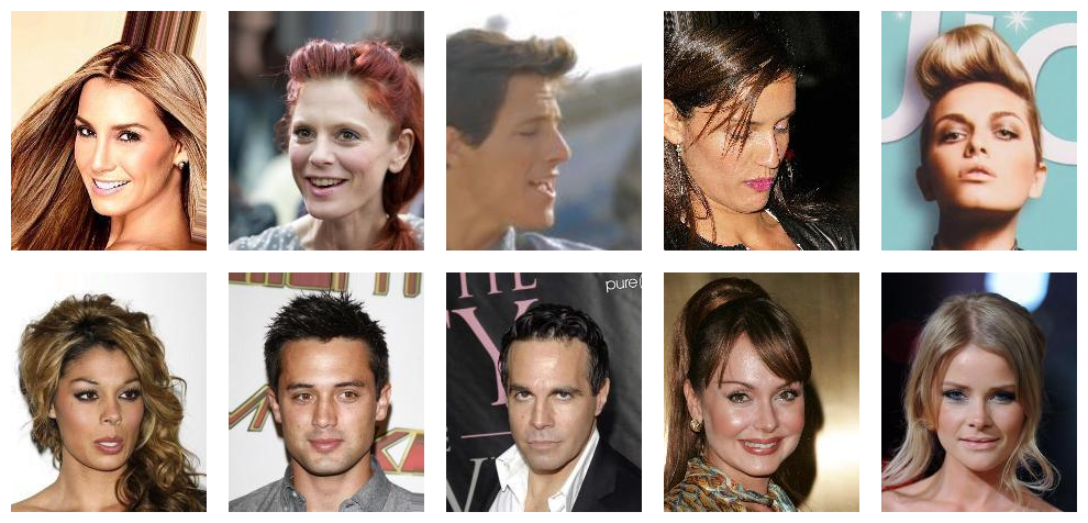
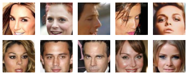
I am going to use CelebA [1], a dataset of 200,000 aligned and cropped 178 x 218-pixel RGB images of celebrities. Each image is tagged with up to 40 different attributes that denote various features like hair color, gender, young or old, smiling or not, pointy nose, etc. See Figure 1 for a preview of the first 10 samples in the dataset, and Table 1 for some example attributes.
| Image | Attributes |
|---|---|
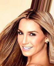 |
Arched eyebrows, attractive, brown hair, heavy makeup, high cheekbones, mouth slightly open, no beard, pointy nose, smiling, straight hair, wearing earrings, wearing lipstick, young. |
 |
5 o’clock shadows, attractive, bags under eyes, big lips, big nose, black hair, bushy eyebrows, male, no beard, pointy nose, straight hair, young. |
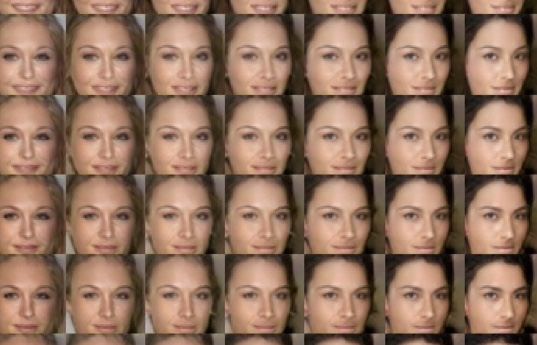
Generative Adversarial Networks are notoriously hard to train on anything but small images (this is the subject of open research), so when creating the dataset in DIGITS I requested 108-pixel center crops of the images resized to 64×64 pixels, see Figure 2. I did not split the data into training and validation sets as I was not interested in measuring out-of-sample performance.
The model I used is straight from DCGAN [2]: the discriminator (D) resembles a typical image classification network with four convolutional layers for feature extraction and one fully connected layer for classification. Likewise, the generator (G) has a symmetrical topology (with transpose convolutions instead of forward convolutions) and identical number of layers and filters. Note that this model is an unconditional GAN and image attributes are not used during training, but I will use them later. See Figure 3 for an illustration of the network topologies.
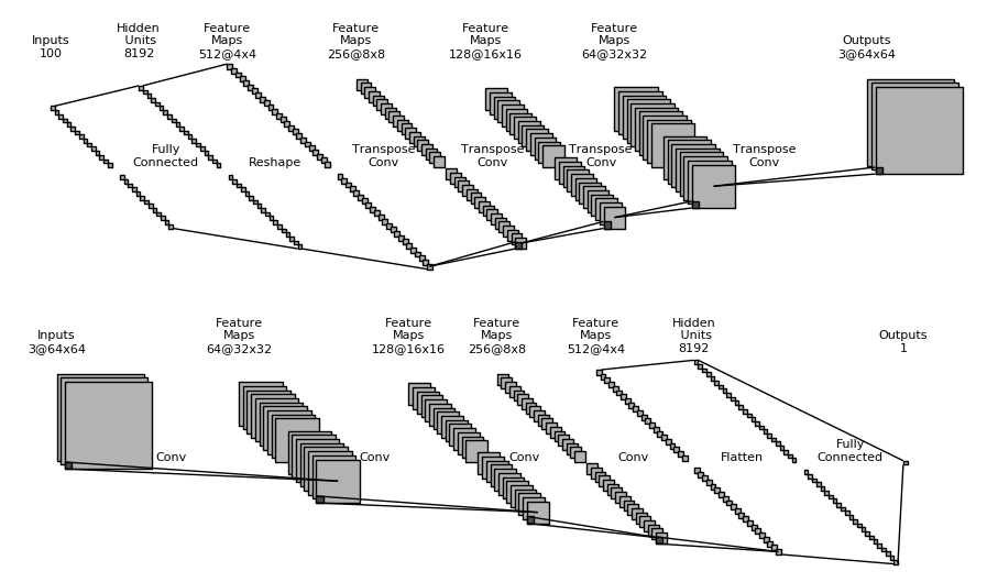
Figure 3: Top: the generator (G) network. Bottom: the discriminator (D) network.On my NVIDIA Titan X board it took 8 hours to train 60 epochs of the 200k-image dataset in DIGITS. I then trained an encoder E using the same method I described in part 1: E is identical to D except for the last layer, which has 100 output neurons to match the length of the latent vector z.
Image Reconstruction with Generative Adversarial Networks
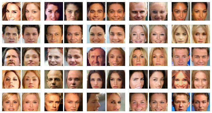
I used my trained models to generate reconstructions of the first 25 images in the dataset. Figure 4 shows the original and reconstructed images. Let’s recap what happened there: I fed each image into E in order to find the corresponding z vector. I then provided the z vector to G in order to get a reconstruction of the image. As you can see, the reconstructions are reasonably good. There are minor failure cases, but in most cases the hair, skin and background colors, the pose, and the shape of the mouth are correctly reconstructed. You can clearly see a bias towards women though, probably because they represent the majority of the dataset. Similarly, it looks like reconstruction works best for faces that look straight into the camera.
Face Attributes
Images in CelebA have 40 binary attributes. I thought it would be nice to be able to take an image of a face and modify it to make it look younger or change the hair color. Remember from part 1 that one of the promises of GANs is that you can perform operations in latent space that are reflected in feature space.
In order to modify attributes, first I needed to find a z vector representing each attribute. So first I used E to compute the z vector for each image in the dataset. Then I calculated attribute vectors as follows: for example, to find the attribute vector for “young” I subtracted the average z vector of all images that don’t have the “young” attribute from the average z vector of all images that have it. I ended up with a 40×100 matrix 
The next step was to create a DIGITS plugin to allow me to choose attributes that I want to add or remove. To edit a face, I need to provide
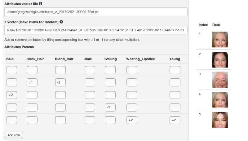
An NVIDIA Titan X GPU can easily generate thousands of these images every second. This makes it possible to interactively actuate the attribute vectors and see in real time how they affect hundreds of face images, as demonstrated in the following video.
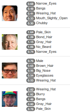
Another fun use of face attributes is to let the model tell us what the main attributes in a face are. Since the images in CelebA are already tagged, it wouldn’t be fair to try this on the dataset, however I thought it would be interesting to try it on real-world images. I used E again to find the z vector for my input image. I then computed the inner product between z and each of the normalized attribute vectors in 
Analogies
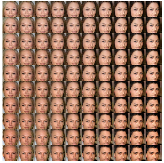
Ever heard about the analogy “king – man + woman = queen”? My GAN-Auto-Encoder framework allows me to perform the same analogies on images, using simple arithmetic in latent space. Have a look at Figure 7 and see for yourself how this works amazingly well in practice (method borrowed from [3]). Table 2 guides you through the process. Take some time to ponder on the beauty of this analogy.
| Male | Blond Hair | Dark Hair | Blue Eyes | Dark Eyes | Smile | Looking Left | Pointy Nose | |
|---|---|---|---|---|---|---|---|---|
| Top Right | + | + | + | + | + | |||
| Bottom Left | + | + | + | |||||
| Subtract Top Left | – | – | – | |||||
| Bottom Right | + | + | + | + | + |
Visualizing the Latent Space
A common way of visualizing the latent space is to project the high-dimensional latent representation onto a 2D or 3D space using Principal Component Analysis or t-SNE. Tensorboard has built-in support for this, making it very easy to display small thumbnails of our images on a sphere, as you can see in the following video. Note how images are nicely clustered according to their main features like the color of the skin or hair. Remember that I trained an unconditional GAN and that image attributes were never given to the network. Yet, the model learned a notion of what makes images similar and how to make them close in latent space. This should convince you about the power of unsupervised learning: the model is able to learn discriminative features of the dataset without ever being told what they are.
A number of applications could derive from the idea that similar samples are close together in latent space. This could be useful for face recognition, signature verification, or fingerprint matching. This could also be a useful stage in a supervised learning pipeline: instead of annotating every single image individually, you could annotate whole regions of latent space. This way you could select hundreds of images at a time to set attributes (people with glasses, etc.).
OpenAI showed in [4] that with a small number of labeled samples, it is possible to leverage the knowledge acquired by a GAN through unsupervised learning and match the performance of fully-supervised models that require orders of magnitude more labeled samples.
Degenerating the Generator
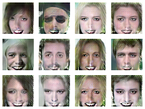
One last thing I would like to show is the outcome of an experiment I ran to check whether gradients were flowing well in my model. After training for a number of epochs, I stopped updating D. I wanted to verify that G’s loss would immediately drop. Indeed it did and besides I noticed that G had degenerated into a state where it would always produce the same face: G had learned to maximize one mode of D. Although the resulting images (Figure 8) are a bit spooky, they seem to capture the essence of the dataset: faces with pale skin, prominent lips, fierce eyes, zebra hair and a fuzzy background! Imagine what kind of images a degenerate G would produce on a dataset of impressionist artists!
Now it’s Your Turn!
After reading this post, you should have the information you need to get started with Generative Adversarial Networks. Download the source code now and experiment with these ideas on your own dataset. Please let us know how you are doing by commenting on this post!
Join NVIDIA for a GAN Demo at ICLR
Visit the NVIDIA booth at ICLR Apr 24-26 in Toulon, France to see a demo based on my code of a DCGAN network trained on the CelebA celebrity faces dataset. Follow us at @NVIDIAAI on Twitter for updates on our ground breaking research published at ICLR.
Learn More at GTC 2017
The GPU Technology Conference, May 8-11 in San Jose, is the largest and most important event of the year for AI and GPU developers. Use the code CMDLIPF to receive 20% off registration, and remember to check out my talk, S7695 – Photo Editing with Generative Adversarial Networks. I’ll also be instructing a Deep Learning Institute hands on lab at GTC: L7133 – Photo Editing with Generative Adversarial Networks in TensorFlow and DIGITS.
Acknowledgements
I would like to thank Taehoon Kim (Github @carpedm20) for his DCGAN implementation on [6]. I would like to thank Mark Harris for his insightful comments and suggestions.
References
[1] Ziwei Liu and Ping Luo and Xiaogang Wang and Xiaoou Tang (2015). Deep Learning Face Attributes in the Wild. Proceedings of International Conference on Computer Vision (ICCV).
[2] Alec Radford, Luke Metz, Soumith Chintala (2015). Unsupervised Representation Learning with Deep Convolutional Generative Adversarial Networks. arXiv:1511.06434
[3] Tom White (2016). Sampling Generative Networks. arXiv:1609.04468
[4] Generative Models. https://openai.com/blog/generative-models/
[5] DCGAN-tensorflow. https://github.com/carpedm20/DCGAN-tensorflow