RTX introduces an exciting and fundamental shift in the way lighting systems work in games and applications. In this video series, NVIDIA Engineers Martin-Karl Lefrancois and Pascal Gautron help you get started with real-time ray tracing. You’ll learn how data and rendering is managed, how acceleration structures and shaders work, and what new components are needed for your pipeline. We’ll also include key slides from the presentation on which this video series is based.
| Part 1: Ray Tracing: An Overview | Part 2: Data and Rendering |
| Part 3: RTX Acceleration Structures | Part 4: Ray Tracing Shaders |
| Part 5: Ray Tracing Pipeline | Part 6: Additional Help |
These videos are rich with information, but don’t worry about jotting things down while you watch; we’ve taken the notes for you. You’ll find the “key things” from every clip presented as bullets. We strongly recommend you watch the videos before digging into the bullets, though, to ensure you are getting the proper context.
Part 1: Ray Tracing: An Overview (3:15 min)
In this video, Martin-Karl offers a quick primer on the difference between rasterization and ray tracing.
Key things from part 1
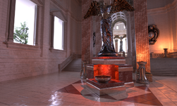
- Ray tracing is a fundamentally different rendering process than rasterization, shown in figure 1.
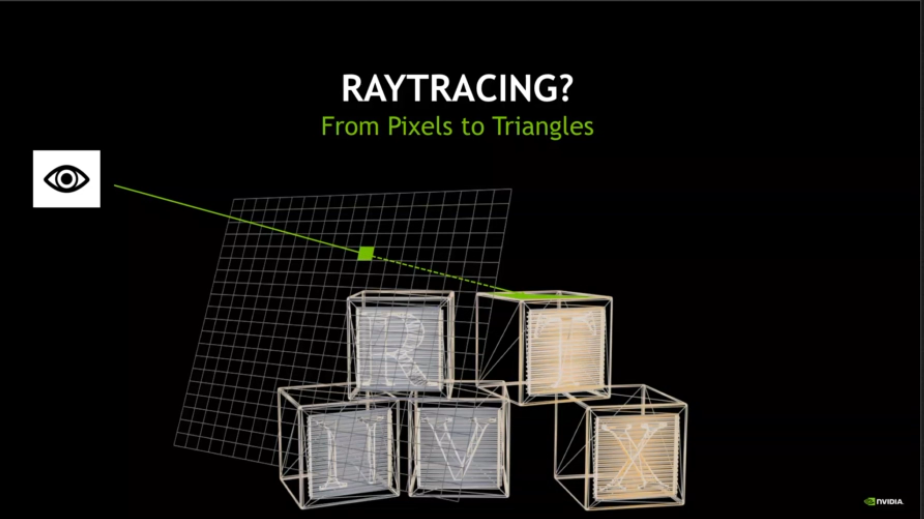
- Further rays can be traced to compute the shading for that pixel.
- When you trace a ray, it hits the closest triangle and returns that to you.
- You don’t have to sort it out. It will just return the closest triangles along that ray.
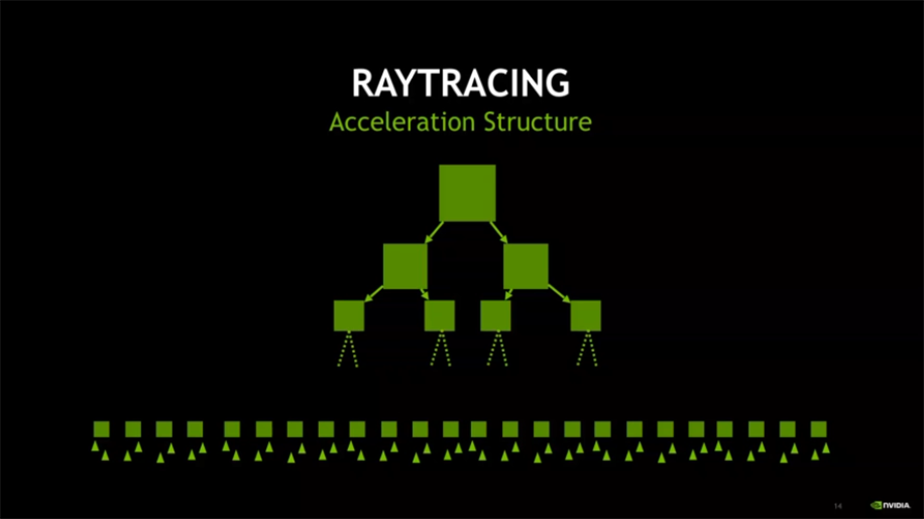
- What happens when you have a lot of triangles in your scene? How can that get processing handled quickly? You need an acceleration structure, shown in figure 2. You have a big bounding box around all of your objects in the scene, and one algorithm will split that box, and do that repeatedly, until the box contains just a few triangles. Then, you’ll be able to test against those triangles.
Part 2: Data and Rendering (11:14 min)
Martin-Karl explains what comprises data in real-time ray tracing, and makes clear how acceleration structures, the pipeline and the binding tables work together.
Key things from part 2
- Graphics programs include UI and interactions, an engine update, data, and rendering. We are specifically interested in the data and rendering components for ray tracing.
- Rasters include buffers of vertices and indices that contain all of the triangles in your scene, as shown in figure 3, as well as your vertex and fragment shaders.
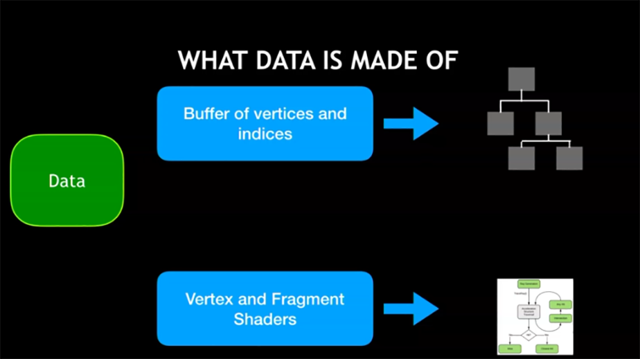
- Together, they will help to draw your scene. In raytracing, you have to convert the buffers of vertices and indices into acceleration structures. Likewise, the vertex and fragment shaders must be converted into a different type of shading system. In a raster, these are separate. In a ray tracer, you have to combine these things.
- The Bottom Level Acceleration Structure (BLAS) and Top Level Acceleration Structure (TLAS) represent two parts. Why is the structure split in this way? Let’s consider an example with a city, a car, and a truck, shown in figure 4.
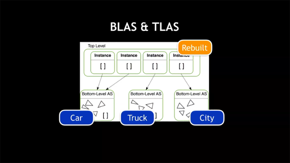
- One acceleration structure holds the city. You place all your buildings inside that. This is all static; you want to render and ray trace that piece very rapidly.
- Another acceleration structure holds the car. In this example, two instances use it because the same car can be a different color in the scene.
- Finally, let’s add a truck using one instance.
- You can easily rebuild the top level. Cars can move throughout the city, and you don’t have to rebuild the entire system.
- You can rebuild in the bottom level. If one structure must adjust – say, a car crashes – you can make that change without having to change the other structures.
- You want to minimize the number of bottom structures for performance reasons. Tracing a ray through two overlapping BLAS requires doing twice the work to find the closest intersection point… it’s important to have that separation.
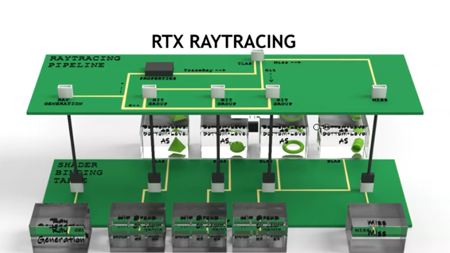
- Let’s take a look at the ray tracing pipeline, seen in figure 5.
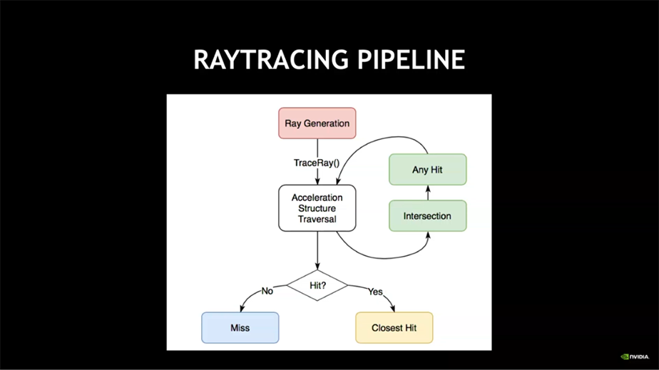
- The pipeline consists of a set of shaders, as outlined in figure 6.
- You start with a pixel that goes to your ray generation shader. That’s where you decide to start and the direction you shoot your ray, a process called ray generation, performed on a per-pixel basis. This will be called for every single pixel you have prepared.
- Then, it will go to the traverse, and call the intersection shader. There is a built-in one for triangles (which can be overridden).
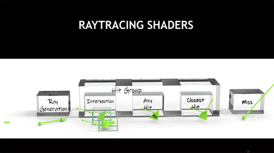
- There is also an any hit shader. This is built into the pipeline but you can override it. For example, a tree with leaves whose shape is defined by an alpha texture. You want the system to go through all the leaves until it really hits something. It tests for alpha, and generates a closest hit only when the leaf body get really touched, not when it just touches the outside of the leaf.
- You can also use this for shadow rays.
- The closest hit shader comes into play when you actually touch the object. Closest hit holds the code for the shading. You can also trace new rays from there and trace it for your shadow.
- The miss shader kicks in when you don’t touch anything. You totally miss all the objects inside your scene. This would be your environment shader, for example.
All together now
The diagram in figure 7 shows the possibilities when you fully use the ray tracing shader pipeline.
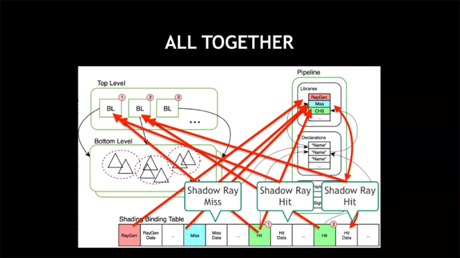
- You have a TLAS (Top Level Acceleration Structure) and a BLAS (Bottom Level Acceleration Structure).
- The pipeline is where you find your compiled shaders and where you declare all your shaders.
- The shading binding table will bind the elements of your shaders.
- Together, they all maintain a complex relationship, but not too complex, as shown in the assembly diagram in figure 8.
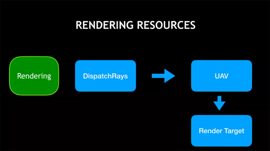
- When it comes to rendering, ray tracing requires just one call,
DispatchRays. Then you can move to UAV, and render target.
Part 3: RTX Acceleration Structures (8:04 min)
Pascal now provides a deeper look into what happens when you try to take your raster-based application and make it work with ray tracing.
Key Things from Part 3
- While the focus of this video series is on Direct X12, the fundamentals all carry over to Vulkan. Read our blog post about how Vulkan ray tracing works with RTX for more details.
Regarding acceleration structures
- Separate the scene into bottom-level instances (BLAS)
- Generate a bottom-level acceleration structure for each instance
- Fewer BLAS is better.
- Keep dynamic objects in their own BLAS.
- Use refitting for dynamic objects
- The generate the top-level acceleration structure (TLAS)
How do we build the BLAS?
- Start from a descriptor, as shown in figure 10.
- You’ll be able to re-use the data used in your raster-based application. Typically, you can point to your vertex and the index buffer, and access the exact same data. You can describe your objects with whatever ranges corresponded to each object in the raster-based application.
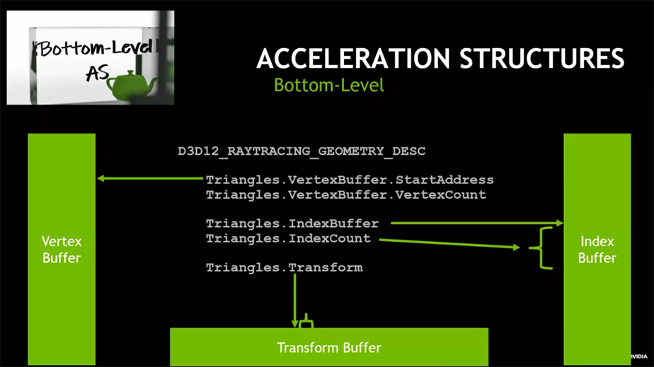
- You can put together different objects in a BLAS and locate them using a transform buffer which will bake them in one acceleration structure.
- The triangles will be internally transformed and put in the right place inside the acceleration structure.
- We build another descriptor that will give us some information on what our BLAS will be. We need to define whether we want to be able to update our structure, as figure 11 shows.
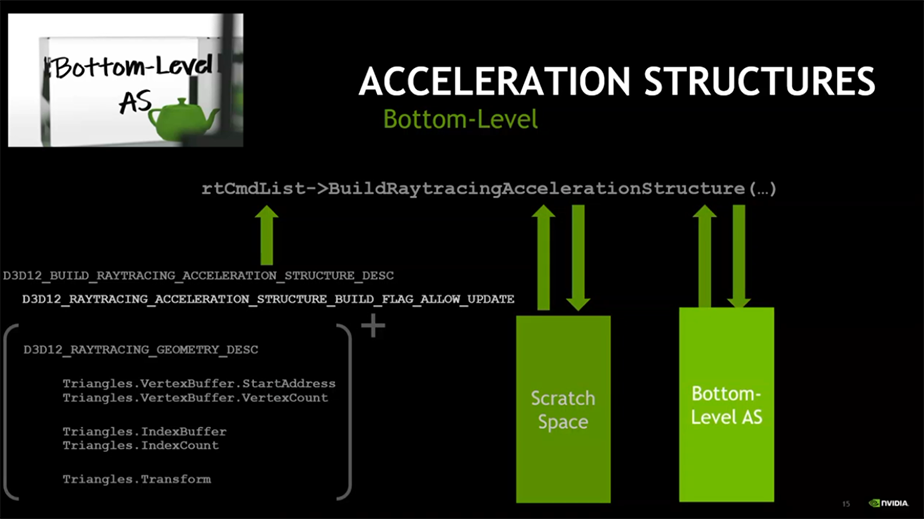
Obtain pre-build information
- Determine the size of the resulting acceleration structure.
- The scratch data size describes how much memory the acceleration structure builder requires for the process of building. You need to allocate this memory.
- In DX12 has no hidden allocation; everything must be done explicitly.
- The scratch space is only used during the build. Afterwards, you can deallocate.
- Once allocate scratch space, you can re-use all the descriptors you had. You can create another descriptor with an update flag for optional refitting. Finally, your BLAS can be built, which happens quickly on the GPU.
Build the TLAS
- It’s like handling a scene graph, only you have two levels.
- Each instance has an ID – something that describes where to find the shader that corresponds to the object, as you can see in figure 12.
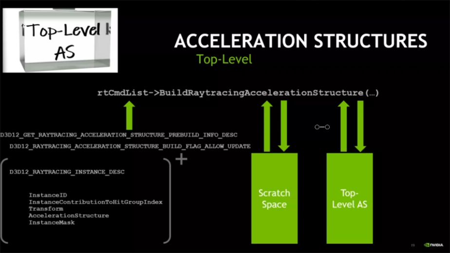
- Again, we have a transform, this time in the TLAS. If we want to move a complete bottom level around in the world, we can use this and have very fast re-fits without having to touch the actual geometry.
- You follow the same principle that you did with the BLAS, but instead of geometry, we’ll be getting instanced information.
Part 4: Ray Tracing Shaders (7:50 min)
Pascal is going to provide a deeper look into what happens when you try to take your raster-based application and make it work with ray tracing.
Key things from part 4
- A ray payload is a structure passed from one shader to another.
- It all happens under the hood in RTX.
- A smaller payload is a lot better!
- The new Direct X compiler allows you to give semantics to your shader.
- You can compile several shaders together, and still know which shaders are useful for what purpose (Figure 13).
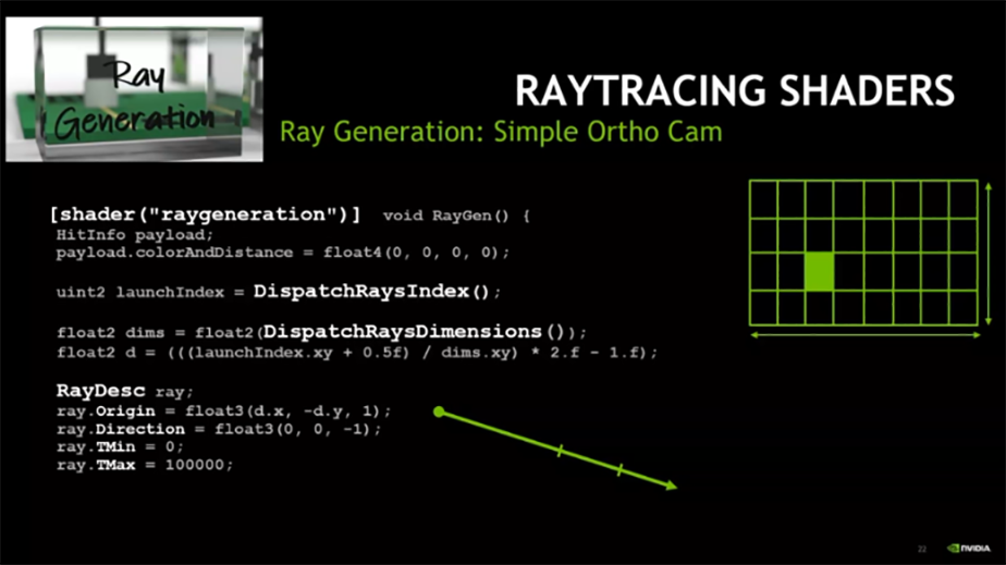
- The dispatch ray index is like the Thread ID in CUDA; it identifies which thread is currently running and the dimensions of the image.
- You describe a ray with origin, direction, and minimum and maximum distance between which we look for intersections.
- Figure 14 shows the need to call a new instruction call,
TraceRay, which takes a few parameters.

TraceRay call.- The first is the TLAS.
- Raymask allows you to mask out some objects. For example, if you decide an object does not cast shadows, the ray mask can be used in conjunction with the instance mask to prevent the ray from intersecting the object.
- Apply a few offsets. The first offset identifies which shader to use for a given object. The second offset describes where in the list of shaders we should start.
- We can have several miss shaders. One may look at the environment, one may return and say, “nothing’s visible”, etc.
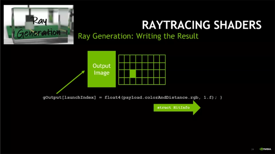
- Finally, we pass our ray and our payload (Figure 15). This payload will directly come back. As soon as we call
TraceRaywe can assume the whole ray tracing has happened and the payload is filled. - You can write the results of your shading directly in the output buffer (Figure 15).
- Avoid recursions! Let the raygen do the heavy lifting. Flattening the recursive ray tracing into a loop in the ray generation results in much less stack management.
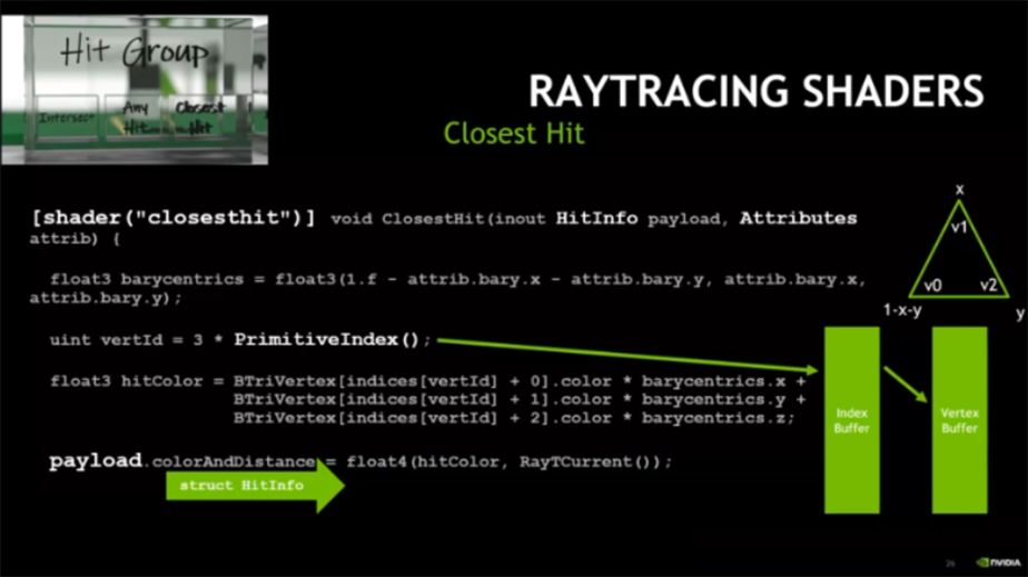
- In raster, you just project your triangles on screen, then interpolate your attributes. RTX gives you the index of the triangle you intersect. You then need to fetch all the attributes yourself and interpolate them, as the code example in figure 16 shows. Note that you need to be able to access the vertex and index buffer of your geometry with whatever layout you decided to have.
- Closest hit shaders can also shoot rays, e.g. shadows.
- You access the primitive index, which yields which triangle has been hit during the rendering; then we can interpolate.
- Then you write the payload, and the shader is finished.
- To avoid recursion, you can have your ray generation carry a slightly bigger payload. The hit will return its hit information (Example: I hit this triangle at that coordinate), then the ray generation can generate another ray from there, and then continue, weighting the contribution of the second bounce, and so on. WIth this process, we end up with less stack management and far less memory traffic.
- The final type of shader is the miss shader.
- The miss shader writes directly into the payload, typically returning a fixed value, which can be anything (figure 17).

Part 5: Ray Tracing Pipeline (8:04 Min)
Pascal provides a deep dive into the structure of a ray tracing pipeline, breaking down the key components.
Key things from part 5
- Now that all shaders have been defined, let’s look at how to assemble that into something that can be rendered. (You are effectively creating an executable of the ray tracing process).
- The ray tracing pipeline in DX12 is made up of a series of sub-objects, illustrated in figure 18. For example, you could have a sub-object for different shaders, a sub-object for how to assemble the shaders together, and so on.

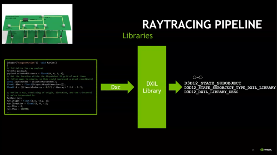
- The first sub-object to look at is the libraries (figure 19).
- You provide your code to the DirectX shader compiler (DXC), which outputs a DLXIL library. That can be run as a sub-object.
- You’ll do that for all the shaders we have.
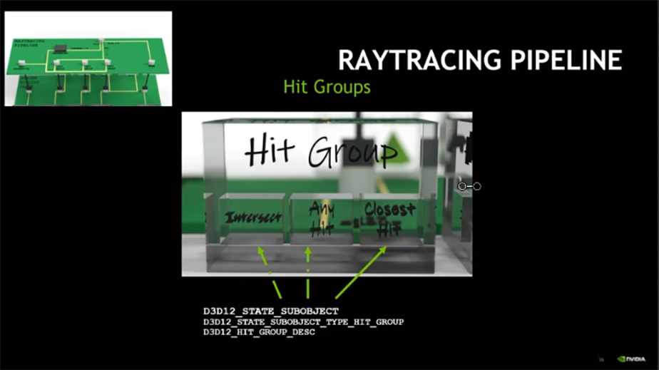
- A Hitgroup describes everything that can happen on one surface for one given type of shader. It includes the intersection shader, any hit, and a close hit shader, shown in figure 20.
- These combine these to give us all the code we need.
- It’s important to note the intersection and any hit shaders. We have some built in to intersect triangles (and to do nothing in the case of an any hit).
- Leave intersection and any hit to nullptr when possible.
- Another sub-object is the shader configuration, which describes the size of the payload you want to use. Shader configurations define sizes of the attributes used for intersections.
- Keep those as small as possible; the built-in intersection shader returns 2 floats.
- Associations in DXR associate shaders with a payload and attribute properties. You need to do this explicitly. Figure 21 illustrates how this can be performed.
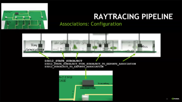
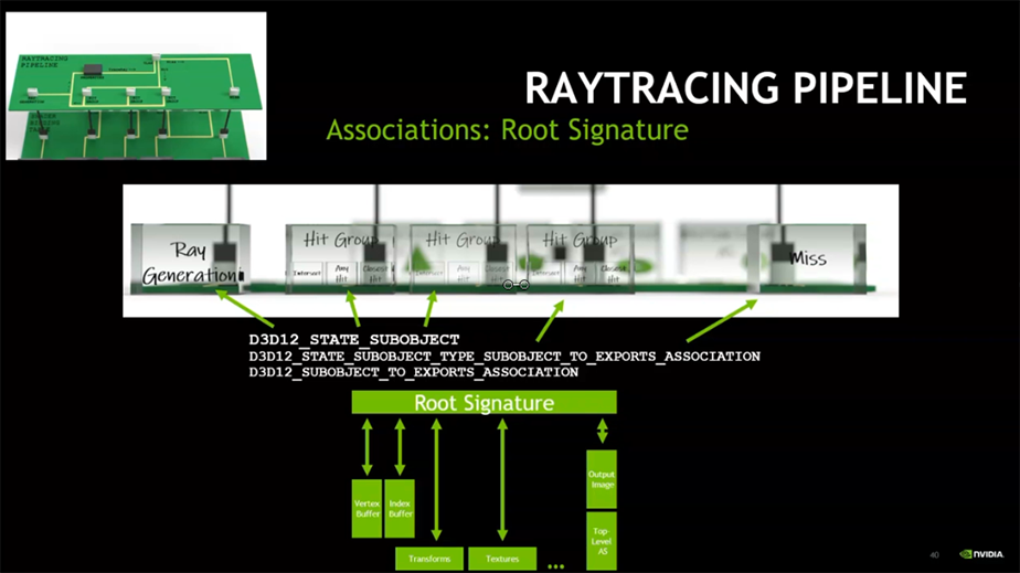
- Each shader in DXR contains a root signature that describes all the resources that will be accessed, shown in figure 22.
- Each shader used needs its own root signature.
- The root signature also goes through an association object.
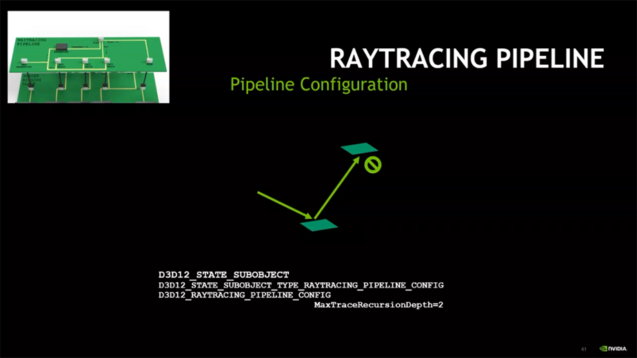
- A pipeline configuration exists that decides how many bounces you can make (figure 23).
- Avoid recursion by flattening into a loop in raygen.
- Now let’s examine the shader binding table, which associates the geometry with the shaders we will execute, outlined in figure 23.
- The shader binding table has a number of entries, a descriptor for the shader, and all the pointers to the external resources.
- It needs to follow the exact layout of the root signature you provided.
- Each shader type requires a fixed size entry.
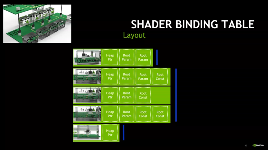
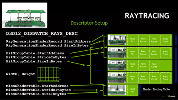
- The descriptor setup determines how we can interpret the shading binding table, as shown in figure 24.
- You need to indicate where you can find the ray generation shader.
- You must define the size of one entry in the ray generation, shader, hit groups and miss shaders
- You must also provide the dimensions of the image to render.
Now that we’ve rendered our first image, let’s think about shadows.
- Here are some simple shader examples for shadow rays, shown in figure 25.
- If we hit something it’s “true”.
- If we do not, it’s “false”.

- In our original closest hit shader, we need to add another trace ray, as you can see in figure 26.
- This time we will offset our hit group to say, “I want the second hit group for the object I’m going to hit, and the second miss, also.”
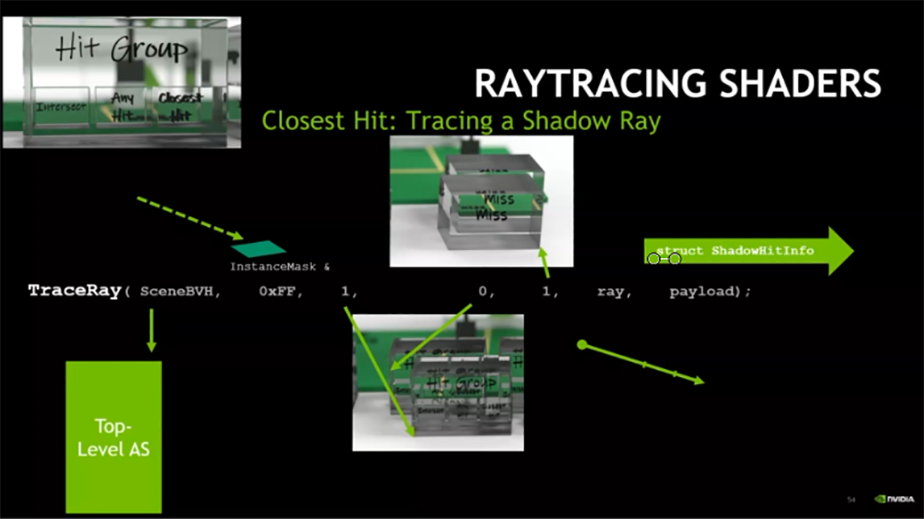
- In our original closest hit shader, we need to add another trace ray.
- This time we will offset our hit group to say, “I want the second hit group for the object I’m going to hit, and the second miss, also.”
Part 6: Additional help with ray tracing (3:47 min)
Martin and Pascal provide guidance on next steps, and detail a range of supporting materials that will help you on your way towards adopting real-time ray tracing in your applications.
NVIDIA will be continuing to build out a “Helper’s Toolbox” for RTX. Additional resources include:
- DXR Blog
- Raytracing links:
- More on NVIDIA RTX
- Getting started ray tracing tutorial
- GameWorks ray tracing overview
- Resources:
- DevTech:
- Pascal Gautron: pgautron@nvidia.com
- Martin-Karl Lefrancois: mlefrancois@nvidia.com