Training with larger batches is a straightforward way to scale training of deep neural networks to larger numbers of accelerators and reduce the training time. However, as the batch size increases, numerical instability can appear in the training process. The purpose of this post is to provide an overview of one class of solutions to this problem: layer-wise adaptive optimizers, such as LARS, LARC, and LAMB. We will also discuss how NVIDIA’s implementation of LAMB, or NVLAMB, differs from the originally published algorithm.
Typically, DNN training uses mini-batch Stochastic Gradient Descent (SGD), which adapts all model weights with a tunable parameter called the learning rate or step size λ in the following way: wt+1 = wt – λ ∗ ∇L(wt), where wt and ∇L(wt) is the weight and the stochastic gradient of loss L with respect to the weight at the current training step t.
When λ is large, the update ||λ ∗ ∇L(wt)|| can become larger than ||wt||, and this can cause the training process to diverge. This is particularly problematic with larger mini-batch sizes, because they require higher learning rates to compensate for fewer training updates. But, training frequently diverges when the learning rate is too high, thereby limiting the maximum mini-batch size we can scale up to. It turns out, based on observations by You et al., that some layers may cause instability before others, and the “weakest” of these layers limits the overall learning rate that may be applied to the model, thereby limiting model convergence and maximum mini-batch size.
Layer-wise Adaptive Approaches
The Layer-wise Adaptive Rate Scaling (LARS) optimizer by You et al. is an extension of SGD with momentum which determines a learning rate per layer by 1) normalizing gradients by L2 norm of gradients 2) scaling normalized gradients by the L2 norm of the weight in order to uncouple the magnitude of update from the magnitude of gradient. The ratio of the norm of the weight to the norm of the gradient is called the trust ratio for each layer. This allows the more stable layers (with larger ||wt||) to use a more aggressive learning rate and often converge more quickly to improve the time-to-solution without a loss in accuracy.
A similar implementation has been developed, named Layer-wise Adaptive Rate Control (LARC), that builds on LARS and includes the option to either clip or scale learning rate based on the trust ratio that is computed similarly to Step 6 in the NVLAMB algorithm below. The LARC implementation is a superset of LARS with an additional option for clipping, and it is available in the NVIDIA APEX PyTorch extension library.
Adam is a member of a category of algorithms inspired by AdaGrad, which normalized the first gradient moment by norm of second moment. Adam introduces running averages of the first two gradients moments: mean and variance. Adam is preferred method to train models for NLP, reinforcement learning, GANs etc. (ref) It was observed that Adam is stable w.r.t. to very noisy gradients, which makes it robust to weight initializations and initial learning rate selection. On the other hand it was observed that Adam does not perform well for training convolutional models used for image classifications or speech recognition for example. It was also observed that Adam has relatively weak regularization compared to SGD with momentum. Loshchilov and Hutter proposed a new version of Adam – AdamW, which decouples weight decay from gradient computation. Please refer to this overview for a more comprehensive comparison of optimizers.
The Layer-wise Adaptive Moments Based (LAMB) optimizer can be seen as the application of LARS to the AdamW optimizer, which adds a per weight normalization with respect to the square root of the second moment to compute the update, as mentioned in the paper. In this article, we will discuss the idea behind NVIDIA’s open-source implementation of LAMB and the adjustments involved to ensure SoTA pretraining convergence results with BERT.
BERT with LAMB
The research article on training BERT with LAMB published on arXiv has four incremental versions. While we started developing our implementation from the first published version of the algorithm (LAMB-v1), our findings led us to a different final algorithm compared to the most recent published version. The goal of the following sections is to help shed some light on the choices made in our implementation. The key differences between all the version is shown in Table 1 below.
| Version | Warmup | Bias Correction | LR decay | Weight Norm Scaling | Gradient Pre-normalization |
| v1 | ✗ | ✓ | poly 1.0 (linear) | ✗ | ✗ |
| v1* | ✓ | ✗ | poly 0.5 | ✗ | — |
| v2 | ✓ | ✗ | poly 1.0 (linear) | ✓ | ✗ |
| v3 | ✓ | ✗ | poly 1.0 (linear) | ✓ | ✗ |
| v4 | ✓ | ✓ | poly 1.0 (linear) | ✓ | ✗ |
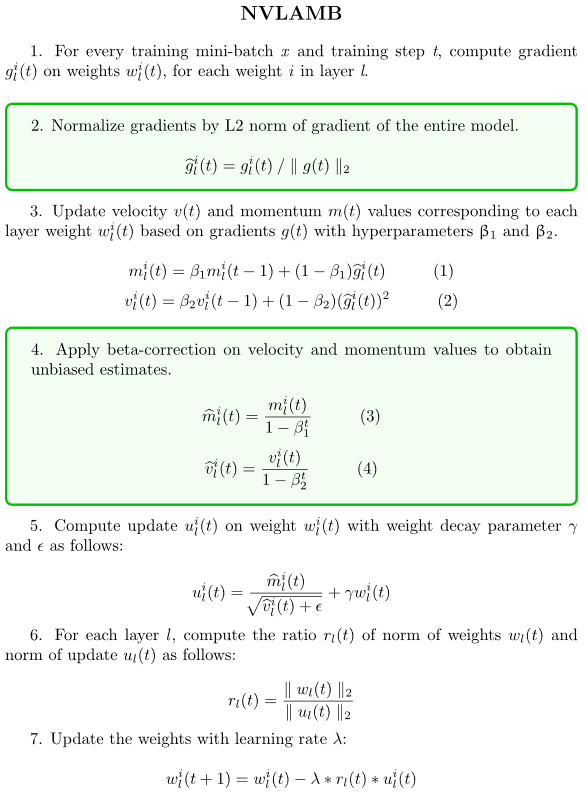
| NVLAMB | ✓ | ✓ | poly 0.5 | ✗ | ✓ |
Table 1. Comparison of LAMB versions to indicate implementation differences. *Direct communication with authors.
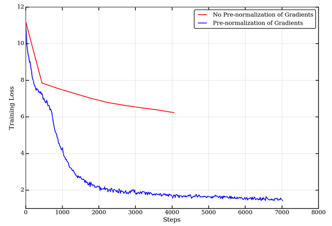
The Importance of Gradient Pre-normalization
We perform a gradient pre-normalization step such that gradients on the entire model combined (all individual layers / weight matrices) are unit L2 norm, as described in Step 2 in the NVLAMB algorithm above. Pre-normalization is important since updates are only dependant on the gradient direction and not their magnitude. This is particularly beneficial in large batch settings where the direction on the gradient is largely preserved. The larger the batch size, the closer the approximation of the (stochastic) gradient is to the true (full-batch) gradient and is less likely to suffer from noisy gradients. While the LAMB publication does not include this, our experiments found that without pre-normalization, BERT pretraining does not converge as expected.
- Google’s original BERT GitHub repository, which uses the unmodified Adam optimizer, also performs gradient pre-normalization.

Additionally, from LAMB-v2 onward, a scaling factor is used on the norm of a weight while computing the weight update. However, the publication doesn’t provide exact guidance on what scaling factor works best. In step 6 of our NVLAMB implementation, we do not scale the norm of the weight, but are still able to achieve state-of-the-art (SoTA) accuracy on downstream tasks as shown in Table 2 below.
Bias Correction
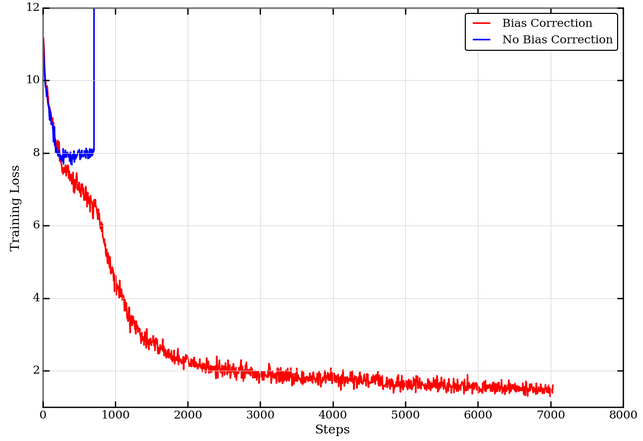
In LAMB-v4, we note the authors use bias correction in the algorithm as well as include learning rate warmup for BERT pretraining. However, a later section in the appendix claims that bias correction can be dropped since its behaviour is similar to warmup.
We experimented further and found that without the correction term, BERT pre-training diverges earlier in the training process, as shown in Figure 3. To understand why this is the case, we observe that initializing the moving averages m and v to zero has an implicit bias of (1 – β1) and (1 – β2) on the subsequent gradients, as shown in Step 3 in the algorithm above. To correct for this factor, the bias correction seen in Step 4 of the NVLAMB algorithm above is necessary. For a more rigorous derivation, please refer to Section 3 in the Adam paper. BERT pretraining uses β2=0.999 and values of β2≈1 required for robustness to sparse gradients result in larger initialization bias. In the case of sparse gradients with values of β2≈1, omitting correction of the bias results in larger updates that often lead to training instabilities and divergence. This has been shown empirically in Section 6.4 in the Adam paper.
Learning Rate Decay
Our experiments show that the degree of learning rate decay makes no observable difference. The accuracy after fine-tuning on downstream SQuAD 1.1 yield identical F1 scores in the range 91 – 91.5 % in both settings.

| Optimizer | Batch Size | Training Steps | Total Samples seen | Squad v1.1 (DEV) F1 | GLUE (Dev) | ||||
| MRPC Accuracy | MNLI-m F1 |
CoLA MCC |
|||||||
| Phase1 | Phase2 | Phase1 | Phase2 | ||||||
| Adam-W (BERT paper) | – | 256+ | – | 1M+ | 256M+ | 90.9+ | 87.3* | 86.13* | 64.8* |
| Adam-W | 65536 | 32768 | 7038 | 1561 | 512M | N/A | N/A | N/A | N/A |
| LAMBv4 | 65536 | 32768 | 7038 | 1561 | 512M | 90.58 | N/A | N/A | N/A |
| NVLAMB | 65536 | 32768 | 7038 | 1561 | 512M | 91.5 | 89.4 | 85.96 | 63.3 |
Table 2. Fine-tuning results on SqUAD v1.1 and GLUE benchmarks.
- scores obtained using published checkpoint
- batch size and training steps as mentioned in BERT
Note 1: Metrics achieved on the best fine-tuning runs on the above checkpoints are reported.
GLUE(Dev) accuracies for Adam-W are obtained by fine-tuning Google’s pretrained checkpoint
Note 2: The LAMB results were obtained using twice the number of training samples as Adam-W, to achieve similar accuracies on downstream fine-tuning tasks as seen in Table 2. The original LAMB publication doesn’t explain how this was determined. We did not attempt to understand whether a different training recipe could use fewer total training samples. This is a potential area for further investigation.
Conclusion
We showcased the general idea behind layer-wise adaptive optimizers and how they build on top of existing optimizers that use a common global learning rate across all layers, and specifically the various published versions of LAMB as well as our implementation of NVLAMB. Layer-wise adaptive optimizer approaches enable training with larger mini-batches with no compromise in accuracy as shown in Table 2. This results in dramatically reduced training times on modern parallel hardware, down from days to almost an hour, as described in our earlier blog. We also provide the implementation in our BERT repositories based on PyTorch and TensorFlow.
Additional Resources
- Learn more about conversational AI
- Large Batch Training of Convolutional Networks
- Adam: A Method For Stochastic Optimization
- Decoupled Weight Decay Regularization
- Understanding the Role of Momentum in Stochastic Gradient Methods
- On Large-Batch Training for Deep Learning: Generalization Gap and Sharp Minima
- ADADELTA: An Adaptive Learning Rate Method
- Large Batch Optimization for Deep Learning: Training BERT in 76 minutes (Older: [v1] [v2] [v3])
- Stochastic Gradient Methods with Layer-wise Adaptive Moments for Training of Deep Networks
- NVIDIA Clocks World’s Fastest BERT Training Time and Largest Transformer Based Model, Paving Path for Advanced Conversational AI
- Large Batch Optimization for Deep Learning: Training BERT in 76 minutes