Optimizing real-time graphics applications for maximum performance can be a challenging endeavor, and ray tracing is no exception. Whether you want to make your graphics engine more efficient overall or find a specific performance bottleneck, profiling is the most important tool to achieve your goals. Despite constantly improving support for ray tracing APIs in profilers such as Nsight Graphics, it is often useful to gain additional performance data through engine instrumentation.
One method that we have found to be particularly effective is the interactive visualization of time spent per pixel as a heatmap during live gameplay. This can directly reveal hotspots caused by expensive geometric situations, shading inefficiencies, and other types of bottlenecks.
By exposing a new lightweight NVAPI intrinsic that lets HLSL shaders query a global high resolution timer, engines can now incorporate such heatmaps with little effort into their debugging or profiling modes.
In this post, we walk you through the necessary steps to get started.


Accessing NVAPI functionality in HLSL
To use NVAPI, download the latest SDK from the NVIDIA NVAPI SDK. To access the timer methods, you need version R440 or later.
NVAPI enables high-resolution timer queries in HLSL shaders through its HLSL extensions. These extensions use a “fake” UAV with special sequences of regular HLSL instructions for communicating to the driver the use of an extension. The special sequences are wrapped in functions such as NvGetSpecial, which we use later in this post.
On the host side, the driver must be made aware of which register slot and space to reserve for the fake UAV sequences. This is done with a simple NVAPI function call before ray tracing shaders are compiled with ID3D12Device::CreateStateObject. The example code in the following section illustrates the process. The fake UAV must be a part of the root signature although no actual resource should be created.
Sample host code
To use NVAPI anywhere in an application, it must be initialized before the first NVAPI call, as shown in the following code example:
#include "nvapi/nvapi.h"

NvAPI_Status NvapiStatus = NvAPI_Initialize();

if(NvapiStatus != NVAPI_OK)
{
    printf( "NVAPI ERROR %d\n", NvapiStatus );
}

// Call NvAPI_Unload() at application exit to un-initialize NVAPI
To inform the driver of the fake UAV slot information that the corresponding shader uses, you must wrap state object creation with NVAPI calls:
// The second parameter is the fake UAV slot index that is used
// in the shader (u1 in this example). The third parameter specifies
// the register space (space0).
//
// NOTE: For multi-threaded shader creation, use
// NvAPI_D3D12_SetNvShaderExtnSlotSpaceLocalThread instead of
// NvAPI_D3D12_SetNvShaderExtnSlotSpace.

NvAPI_Status NvapiStatus = NvAPI_D3D12_SetNvShaderExtnSlotSpace( state->device.Get(), 1, 0 );

if(NvapiStatus != NVAPI_OK)
{
    printf( "NVAPI ERROR %d\n", NvapiStatus );
}

// Create ray tracing state objects or collections.
// Note that for shader compilation to succeed, the fake UAV slot
// must also be part of the root signature. No actual resource or
// descriptor has to be created, however.
D3Ddevice->CreateStateObject( ... );

// Disable the NVAPI extension slot again after state object creation.
NvapiStatus = NvAPI_D3D12_SetNvShaderExtnSlotSpace( state->device.Get(), ~0u, 0 );

if(NvapiStatus != NVAPI_OK)
{
    printf( "NVAPI ERROR %d\n", NvapiStatus );
}
Sample HLSL code
Any shader that uses NVAPI HLSL extensions must #define the NV_SHADER_EXTN_SLOT and NV_SHADER_REGISTER_SPACE macros and then #include nvHLSLExtns.h.
The UAV slot and register space must match the host code shown earlier, so we use slot 1 and space 0. The format must be the same as shown below, “u<slot #>” and “space<space #>”. Avoid using slot 0, as it may be reserved.
#define NV_SHADER_EXTN_SLOT u1
#define NV_SHADER_EXTN_REGISTER_SPACE space0
#include "nvapi/nvHLSLExtns.h"
You can now use NvGetSpecial to access the timer registers and begin peppering your shaders with queries, for example before and after a TraceRay call. Then, use some helper functions to compute a heatmap color based on the time deltas:
// Get timer value
uint startTime = NvGetSpecial( NV_SPECIALOP_GLOBAL_TIMER_LO );
...
TraceRay( ... );
...
uint endTime = NvGetSpecial( NV_SPECIALOP_GLOBAL_TIMER_LO );
uint deltaTime = timediff( startTime, endTime );

// Scale the time delta value to [0,1]
static float heatmapScale = 65000.0f; // somewhat arbitrary scaling factor, experiment to find a value that works well in your app
float deltaTimeScaled =  clamp( (float)deltaTime / heatmapScale, 0.0f, 1.0f );

// Compute the heatmap color and write it to the output pixel
outputBuffer[DispatchRaysIndex().xy] = temperature( deltaTimeScaled );
For simplicity and to reduce register pressure, this example only used the “LO” counter to obtain the least significant 32 bits of the value, rather than combining LO and HI for a 64-bit result. This is good enough for a heatmap visualization if you account for a single overflow with a helper function like the following code example:
uint timediff( uint startTime, uint endTime )
{
  // Account for (at most one) overflow
  return endTime >= startTime ? (endTime-startTime) : (~0u-(startTime-endTime));
}
There are many ways to map the time delta value computed earlier to pixel colors. Here is the method used for the images in this post:
inline float3 temperature(float t)
{
    const float3 c[10] = {
        float3(   0.0f/255.0f,   2.0f/255.0f,  91.0f/255.0f ),
        float3(   0.0f/255.0f, 108.0f/255.0f, 251.0f/255.0f ),
        float3(   0.0f/255.0f, 221.0f/255.0f, 221.0f/255.0f ),
        float3(  51.0f/255.0f, 221.0f/255.0f,   0.0f/255.0f ),
        float3( 255.0f/255.0f, 252.0f/255.0f,   0.0f/255.0f ),
        float3( 255.0f/255.0f, 180.0f/255.0f,   0.0f/255.0f ),
        float3( 255.0f/255.0f, 104.0f/255.0f,   0.0f/255.0f ),
        float3( 226.0f/255.0f,  22.0f/255.0f,   0.0f/255.0f ),
        float3( 191.0f/255.0f,   0.0f/255.0f,  83.0f/255.0f ),
        float3( 145.0f/255.0f,   0.0f/255.0f,  65.0f/255.0f )
    };

    const float s = t * 10.0f;

    const int cur = int(s) <= 9 ? int(s) : 9;
    const int prv = cur >= 1 ? cur-1 : 0;
    const int nxt = cur < 9 ? cur+1 : 9;

    const float blur = 0.8f;

    const float wc = smoothstep( float(cur)-blur, float(cur)+blur, s ) * (1.0f - smoothstep(float(cur+1)-blur, float(cur+1)+blur, s) );
    const float wp = 1.0f - smoothstep( float(cur)-blur, float(cur)+blur, s );
    const float wn = smoothstep( float(cur+1)-blur, float(cur+1)+blur, s );

    const float3 r = wc*c[cur] + wp*c[prv] + wn*c[nxt];
    return float3( clamp(r.x, 0.0f, 1.0f), clamp(r.y,0.0f,1.0f), clamp(r.z,0.0f,1.0f) );
}
Example: timing primary rays
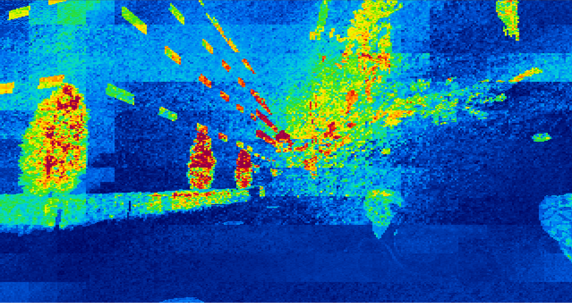
The images in Figure 2 show an example of timing primary rays in the “Bistro” test scene. There are a couple of interesting effects to observe. To better point them out, here’s the same heatmap image with annotations:

Region 1: The most expensive regions in the image are around fine geometric details like tree leaves. This is expected, because more detail means that rays must traverse further down the bounding volume hierarchy (BVH) to locate the actual triangles to intersect. In addition, due to the somewhat chaotic geometric situation in those areas, triangle bounding boxes often overlap, requiring an increased number of box and triangle tests per ray compared to more structured geometry. This effect can be mitigated if content creators (and content tools) are aware and aim to avoid meshes with overlapping primitives, as well as other suboptimal configurations like triangle fans and long, thin triangles.
Region 2: Because the street facade is almost parallel to the viewing direction, many rays in this region graze along geometry that they barely miss before hitting anything. This grazing increases the cost of tracing a ray, because the BVH must be examined at a fine-grained level just to determine that the ray misses and the intersection search must continue. This effect is quite fundamental to the way ray tracing works and is typically not possible to avoid entirely.
Region 3: All the balcony panels light up as hot spots, indicating that they are more expensive to trace against than the geometry immediately surrounding them (walls, windows, and so on). This could be a content problem that should be investigated. Potential issues to check for include triangle duplicates, bad tessellation, or missing OPAQUE flags in this part of the scene.
Region 4: An interesting effect visible across the entire image and highlighted in the bottom left corner is the general blocky appearance of the heatmap. This has to do with the fact that the GPU hierarchically splits its work into tiles for better coherence. Multiple tiles are processed in parallel. Depending on which part of the GPU is under load at any given time, executing one tile might affect the runtime of another. This leads to a certain “smearing” of tile costs around expensive areas. It is not something that the application needs to address, but being aware of the effect helps with focusing on the right hotspots.
Conclusion
Timing heat maps are easy to implement and extremely useful to quickly spot ray tracing performance hotspots. Several shipping games have identified important issues using this method, and they were often simple fixes. Examples include pinpointing needlessly expensive geometric situations similar to the test scene in Figures 2 and 3, but also inefficient shaders, missing OPAQUE flags, and others.
We recommend that every graphics engine using ray tracing should include a heatmap mode. In engines that do not trace primary rays by default, it is usually worthwhile to implement a primary ray camera for debugging and profiling purposes.
There are many ways that you can use the new NVAPI timing intrinsic, such as visualizing time for primary or secondary rays, with and without shading, and even timing non-raytracing shaders. Using heat map profiling in your graphics engine not only helps spot concrete issues, it can also help develop a better intuition for where performance is spent in ray tracing.