The NVIDIA Transfer Learning Toolkit is now NVIDIA TAO Toolkit.

It’s important for the model to make accurate predictions when using a deep learning model for production. How efficiently these predictions happen also matters. Examples of efficiency measurements include electrical engineers measuring energy consumption to pick the best voltage regulator, mechanical engineers timing inference latency to determine motor control loop maximum speed, embedded software engineers needing to fit an inference engine into tight memory constraints, and corporate finance estimating cost of a prediction to assess profit potential.

The NVIDIA Transfer Learning Toolkit provides a key feature known as model pruning which addresses these concerns. Pruning has been used to reduce the complexity of neural networks for a long time, as demonstrated by the acclaimed Optimal Brain Damage (OBD) [1] paper in year 1990. The term pruning borrows from the analogous technique used in decision trees, which derives from the horticultural practice of pruning trees.

Trees often carry large numbers of dead branches which produce neither leaves nor fruit and yet cause the tree to be unnecessarily heavy. These dead branches can be safely cut without affecting lead branches, which in most cases benefit from the extra room. Likewise, you may remove unnecessary connections in a neural network so that the corresponding computation does not need execute, freeing up memory, time, energy and money.

Pruning commonly allows reducing the number of parameters by an order of magnitude in the vision applications targeted by TLT, leading to a model that is many times faster.

1. Removing Unnecessary Connections

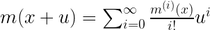
We’ll take a look how to identify which connections to be pruned later. First, let’s look at how the removal can take place in practice and why it is useful. Consider the neural network illustrated on Figure 1 – you might recognize a Multi-Layer Perceptron[2] (MLP) there. This consists of six inputs, one hidden layer of four neurons and two outputs. I need to perform six Multiply-Accumulate (MLA) operations in order to compute the activation of each neuron in the hidden layer. Computing each output requires four MLAs. In total, (2×4)+(4×6)=32 MLAs which need to be executed and 32 parameters (weights) to store in memory.

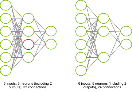
Pruned neuron diagram — Figure 1: Removing one entire neuron. Left: the unpruned neural network with a neuron in red that is thought to be unnecessary. Right: the equivalent pruned neural network, whose computational complexity is 25% smaller.

Assume that by some magical process, I determine that the red neuron in the hidden layer can be entirely removed without dramatically affecting the outputs of my neural network. I now have only (2×3)+(3×6)=24 MLAs. This reduces the computational complexity and memory needed to store parameters by 25%.

I used some approximations above to make my point, so let’s review again the math behind calculating the activation $x_{l,i}%0$ of a neuron $i%0$ within a layer $l%0$ in an MLP, given an activation function $\phi%0$ a weight vector $w_{l,i}%0$ and a bias term $b_{l,i}%0$ :

$x_{l,i} = \phi(\sum_{j}{w_{l,i,j}}x_{l-1,j}+b_{l,i})%0$

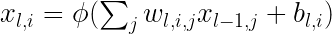
The above formula shows the most computationally intensive term is the summation of the weighted inputs.

Multiple ways exist to prune a neuron $k^*%0$ in this layer:

Consider that some elements within the summation need not be evaluated, i.e. $w_{l,k^*,j}=0%0$ for some values of $j%0$ . Benefiting from this approximation requires excellent support for sparse arithmetics, which is unusual in Deep Learning frameworks.
Also consider that all elements of the summation can be ignored, i.e. $w_{l,k^*,j}=0%0$ for all values of $j%0$ , in which case we can write $x_{l,k^*} = \phi({b_{l,k^*}})%0$ . This removes the summation entirely, reducing the computational complexity substantially but requiring forward propagating the bias term $b_{l,k^*}%0$ .
The bias term and its non-linear transformation by $\phi%0$ may be ignored, in which case we have $x_{l,k^*}=0%0$ , which is a gross approximation but simplifies things immensely.

Transfer Learning Toolkit to simply ignores bias terms. The main reason we do this is that it is straightforward to implement in any Deep Learning framework. We can merely create a clone of the original model with one less neuron in layer $l%0$ and copy all the retained weights $w_{l,i,j}%0$ and bias terms $b_{l,i}%0$ for $i \neq k^*%0$ into the cloned model. I’ll show you why this crude approximation does not hurt a great deal in practice in a later section.

I just described how pruning works in a fully-connected layer. However the model templates we provide in Transfer Learning Toolkit consist of Convolutional Neural Networks for the most part and operate on multi-channel images. How do we prune a convolutional layer?

Remember that given a fixed input size of $c_{in}%0$ channels, $h%0$ rows and $w%0$ columns, a 2D convolutional layer of $c_{out}%0$ filters with a filter size of $m \times n%0$ is functionally identical to a fully-connected layer of $c_{out}%0$ neurons for which each neuron would have its free parameters repeated as many times as it takes to sweep the entire input. In other words, this is a layer with a very large number of connections to the previous layer, and a relatively small number of free parameters $c_{in} \times c_{out} \times m \times n%0$ in total, plus $c_{out}%0$ bias terms). We explained above how we prune entire neurons in fully-connected layers. By analogy, we also prune entire filters in convolutional layers.

2 Selecting Unnecessary Neurons

The previous paragraph explains how to remove neurons but I have not yet explained how to pick them.

2.1 Data-Driven Methods

Identifying the least useful neuron in a neural network with certainty means removing each neuron from the model, one by one, then evaluating the model again on my validation dataset, picking the neuron whose removal led to the best validation metric. If I have a thousand neurons in my model, I need to run a thousand evaluations. Even running these evaluations in parallel means repeating this process sequentially for as many times as there are neurons to remove. Doing so would be very laborious. Making the process of eliminating neurons tractable requires me to make some approximations.

Identifying prunable neurons was already a concern almost 30 years ago when the OBD paper was published. This suggests building an analytical model to determine the impact of a small perturbation of the parameters on the evaluation metric, averaged over all the data in the validation set. The issue is the lack of a closed-form formula for this model.

The paper hints that we can instead calculate a local approximation of the metric $m(x + \delta u)%0$ where $m%0$ is our metric function, $x%0$ is the current value of neural network parameters, and $u%0$ is the small perturbation to apply to the parameters (in our case, setting the weights of one neuron to 0). Such approximations are typically carried out using Taylor expansions in the form:

$m(x+u) = \sum_{i=0}^{\infty}\frac{m^{(i)}(x)}{i!}u^{i}%0$

Where $m^{(i)}%0$ is the $i%0$ th derivative of function $m%0$ . Since we only care about in how our metric varies with $u%0$ , all we need to consider are the derivatives of this function. Interestingly, the OBD paper claims that, since it is assumed that the network has already converged and hit a local minimum, then the first-order derivatives should be close to zero and the second-order derivatives carry most of the information.

Conversely, the authors of a more recent paper [3] claim that while first-order derivatives may be expected to be close to zero on average, they still retain a fair amount of variance that can serve as a great indicator of whether removing a given neuron hurts. Because second-order are hard to compute (due to lack of support in virtually all Deep Learning frameworks), first-order derivatives should be used instead, since they are conveniently calculated during back propagation when training the model (but on the training set, not the validation set!). Both methods are still somewhat complex to implement. Besides, it is difficult to assess whether the noise added by these approximations outweighs the benefits of making them.

Another data-driven heuristic is based on the intuition that unimportant neurons exhibit small-magnitude activations. The implementation is straightforward: I feed all the validation data to my model and record the output of every neuron. Those that have the smallest output can be pruned. Besides, I don’t even need labels. However, is the intuition valid? One neuron may have a large output but if subsequent layers have very small weights on the neuron activation, the neuron brings little contribution to the final output overall. Conversely, a neuron may have a small output which could be amplified in subsequent layers.

2.2 Non Data-Driven Methods

Now let me introduce the most trivial neuron selection method, based on the intuition that neurons that have the smallest weights in magnitude are the least important ones. This is utterly simple, I don’t even need data! Similar to activation-based neuron selection there is no reason for this to be the case in theory, unless I introduce a key modification to the learning schedule: by penalizing neurons for having large weights. This technique is commonly used and referred to as weight-decay regularization and consists of adding a term to the total loss $L_{total}%0$ to optimize:

$L_{total} = L + \lambda \sum_{i}{\parallel W_i \parallel}%0$

$L%0$ is the main loss function and $W_i%0$ are the weights of the model. Adding regularization changes everything; only the neurons which contribute to the main loss are allowed to have large weights.

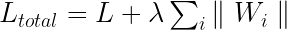
I can implement this method using a script that runs outside of my training loop and just inspects the weights and prunes all the neurons whose norm is below an arbitrary threshold $t%0$ . In other words, an API looks like:

pruned_model = TLT.prune(model, t)

Other considerations need to be taken here so the TLT.prune API takes optional parameters.

One parameter specifies the granularity at which we prune neurons in every layer. The number of neurons in each layer within the model templates is a nice power of 2. This stems from the fact that utilization of GPU compute units is usually maximized for workflows that execute $2^N%0$ times in parallel. Since reducing the number of filters from 32 to 31 might not save much time, the default granularity sets to 8 in the tlt-prune, which enforces that this will not happen.

In the case of convolutional layers, for example, the norm of a filter depends on the size of the filter. A 3×3 filter is likely to have a greater norm than a 1×1 filter. In order to make the pruning threshold comparable across layers, we divide the norm of each neuron by either the norm of the biggest neuron (default) or by the average norm, within a layer. The optimizer argument to tlt-prune can be used to override the default setting.

2.3 Handling Element-Wise Operations of Multiple Inputs

One further complication exists that I haven’t mentioned about the process of identifying the neurons to prune. This one arises in the presence of element-wise operations of multiple inputs.

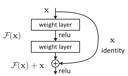
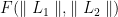
For example, let’s look at residual networks. Several variants are included in the TLT templates, in which an identity shortcut connection propagates attenuated information towards the output of the network. Figure 1 shows that an element-wise addition is used to perform a sum of the identity $x%0$ and the residual block $F(x)%0$ . What happens if I prune neurons off the bottom weight layer? In the general case, I can longer compute the sum $x%0$ and $F(x)%0$ because their shapes differ. Even if the shapes match because $x%0$ has also been pruned, I need to be able to say with 100% confidence that I pruned matching neurons; otherwise the summation no longer makes sense. Every neuron has a corresponding neuron in each of the other inputs of the summation and all of them need to be pruned identically.

Residual block diagram — Figure 2: A residual block. Source.

The way I do this in practice is through a method named equalization. First, I choose an equalization operator. My operator can be any multivariate commutative operator. For example:

Arithmetic mean. $F(x_1 \dots x_n) = \sum{x_n}/N%0$ . This operator prunes a neuron if the average norm of all corresponding neurons across the inputs of the element-wise operation is below the pruning threshold.
Geometric mean. $F(x_1 \dots x_n) = \prod{x_n}^{1/N}%0$ . This is similar to the above operator, except that the geometric average is used.
Union. $F(x_1 \dots x_n) =t \quad if \quad \exists x_n, x_n >= t \quad else \quad t - \epsilon%0$ . A neuron is pruned if the norm of at least one of the corresponding neurons is below the threshold.
Intersection. $F(x_1 \dots x_n) =t \quad if \quad \forall x_n, x_n >= t \quad else \quad t - \epsilon%0$ . The norms of all corresponding neurons must be below the threshold.

I need to find the prunable layers that immediately precede the element-wise operation in the presence of a sum, subtraction product, or any other element-wise operation over multiple input layers. Prunable layers consist of the layers that have neurons and potentially change the shape of tensors. Non-prunable layers are layers such as activation layers.

Suppose there are two input layers $L_1%0$ and $L_2%0$ of $K%0$ neurons each. After I have computed the norms of their neurons I have two vectors $\parallel L_1 \parallel%0$ and $\parallel L_2 \parallel%0$ . My equalization operator gives me another vector $F(\parallel L_1 \parallel, \parallel L_2 \parallel) %0$ that I use to overwrite the norms of my layers. After I have done this I have enforced that the two layers have the same norm. Hence, they are pruned identically and I no longer need to worry about the element-wise operation.

I will traverse the neural network from input to output in three passes:

In the first pass, I compute the norm of each neuron.
In the second pass, I am looking for element-wise operations. If I find one I equalize the norms of its prunable inputs.
In the third pass, I remove all neurons whose norm is below the threshold $t%0$ .

3 Defining a Training Schedule

As mentioned before, I need to train with a fair amount of weight-decay regularization in order to use the non-data driven method to select neurons to prune. In general, I pick a value of $\lambda %0$ that causes the penalization term $\lambda \sum_{i}{\parallel W_i \parallel} %0$ to roughly equal the main loss $L%0$ . Using the default pruning normalizer and a threshold of 10% usually leads to acceptable pruning ratios.

Immediately after pruning, I can evaluate the smaller model again on my validation dataset. Several cases could occur:

The metric barely changes. This is what I observe in the majority of cases. Despite removing many neurons, the model performs equally well.
The metric improves. This occurs relatively rarely, but pruning is another regularizer which may help combat overfit and improve the model’s ability to generalize.
The metric has deteriorated. A dramatic loss of accuracy is sometimes observed. This may happen if we accidentally removed a useful neuron. However, if I keep training my model I can see that the model quickly recovers in the large majority of cases, performing as well as the original model.

In the general case, I do not know which of the three above cases will occur after pruning. Therefore my typical training schedule looks as follows:

Train with aggressive weight-decay regularization
Prune
Re-train

4 Why not train the smaller model in the first place?

If we can remove 90% of the weights in a neural network and retain the original accuracy, why don’t we just train the smaller one in the first place? Indeed, the smaller network would train in a fraction of the time and we wouldn’t need to implement pruning at all. Training the large network sounds like overkill.

The truth is, it’s very hard to train a small model and reach the accuracy of the bigger one. This boils down to something that sounds very simple in principle: the initialization of the weights. Take a look at a fascinating paper on this subject named The Lottery Ticket Hypothesis [5]. The paper hypothesis is that within a big model there is a smaller model that, if trained on its own, would match the performance of the larger one. The issue, however, is that it’s virtually impossible to determine what the smaller model is before training the larger one to completion. The analogy used by the authors is that the random initializations used in our models are like lottery tickets: if you have many of them you stand a good chance at winning the lottery but if you only have a handful, you would have to be incredibly lucky.

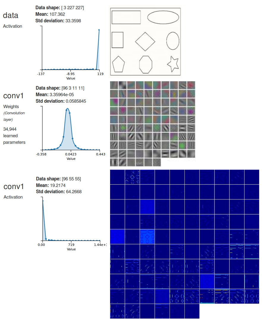
The image in the middle of figure 3 is shows a representation of the filters in the first convolutional layer of a trained AlexNet. You can see that a lot of the filters are all grey, indicating that they are small in magnitude, and the image at the bottom is showing that their activations are also very small. It looks as if these filters did not learn anything. According to the hypothesis in [5] that would be an indication that these unlucky filters merely got an unfavorable initialization.

Weights visualization charts — Figure 3: Visualizations of the weights in the first convolutional layer of AlexNet, trained on ImageNet. The image at the top is showing a sample input image. The image in the middle is showing the weights of the 96 11×11 convolutional filters in the first layer. The image at the bottom is showing the activations of the 96 filters.

NVIDIA Transfer Learning Toolkit provides an end to end deep learning workflow for accelerating deep learning training and deploying with DeepStream SDK 3.0 on Tesla GPUs. Transfer Learning Toolkit for Intelligent Video Analytics (IVA)TLT is now open for early access. If you’d like to try out TLT, please go to the developer early access program at Transfer Learning Toolkit for IVA.