By now, hopefully you read the first two blogs in this series “Migrating to NVIDIA Nsight Tools from NVVP and Nvprof” and “Transitioning to Nsight Systems from NVIDIA Visual Profiler / nvprof,” and you’ve discovered NVIDIA added a few new tools, both Nsight Compute and Nsight Systems, to the repertoire of CUDA tools available for developers. The tools become more and more important when using newer GPU architectures. For the example project in this blog, using the new tools will be necessary to get the results we are after for Turing architecture GPUs and beyond.
As covered previously, Nsight Compute and Nsight Systems differ in their purpose and functionality, so profiling activities will be accomplished in one or the other of these new tools. One of the main purposes of Nsight Compute is to provide access to kernel-level analysis using GPU performance metrics. If you’ve used either the NVIDIA Visual Profiler, or nvprof (the command-line profiler), you may have inspected specific metrics for your CUDA kernels. This blog focuses on how to do that using Nsight Compute. Many of the other profiler activities you may be interested in (e.g. inspecting timelines, measuring activity durations, etc.) can be performed using Nsight Systems.
Getting Started
We’re going to analyze a code that is a variant of the vector add code that was used in the previous blog. In this case, we’ll be looking at a CUDA code that does a matrix-matrix element-wise add operation, effectively a vector add, but using a 2D CUDA grid configuration, along with 2D (i.e. doubly-subscripted) array access. The code is still quite simple:
#include

const size_t size_w = 1024;
const size_t size_h = 1024;

typedef unsigned mytype;
typedef mytype  arr_t[size_w];
const mytype A_val = 1;
const mytype B_val = 2;

__global__ void matrix_add_2D(const arr_t * __restrict__ A, const arr_t * __restrict__ B, arr_t * __restrict__ C, const size_t sw, const size_t sh){

  size_t idx = threadIdx.x+blockDim.x*(size_t)blockIdx.x;
  size_t idy = threadIdx.y+blockDim.y*(size_t)blockIdx.y;

  if ((idx < sh) && (idy < sw)) C[idx][idy] = A[idx][idy] + B[idx][idy];
}

int main(){

  arr_t *A,*B,*C;
  size_t ds = size_w*size_h*sizeof(mytype);
  cudaError_t err = cudaMallocManaged(&A, ds);
  if (err != cudaSuccess) {std::cout << "CUDA error: " << cudaGetErrorString(err) << std::endl; return 0;}
  cudaMallocManaged(&B, ds);
  cudaMallocManaged(&C, ds);
  for (int x = 0; x < size_h; x++)
    for (int y = 0; y < size_w; y++){
      A[x][y] = A_val;
      B[x][y] = B_val;
      C[x][y] = 0;}
  int attr = 0;
  cudaDeviceGetAttribute(&attr, cudaDevAttrConcurrentManagedAccess,0);
  if (attr){
    cudaMemPrefetchAsync(A, ds, 0);
    cudaMemPrefetchAsync(B, ds, 0);
    cudaMemPrefetchAsync(C, ds, 0);}
  dim3 threads(32,32);
  dim3 blocks((size_w+threads.x-1)/threads.x, (size_h+threads.y-1)/threads.y);
  matrix_add_2D<<<blocks,threads>>>(A,B,C, size_w, size_h);
  cudaDeviceSynchronize();
  err = cudaGetLastError();
  if (err != cudaSuccess) {std::cout << "CUDA error: " << cudaGetErrorString(err) << std::endl; return 0;}
  for (int x = 0; x < size_h; x++)
    for (int y = 0; y < size_w; y++)
      if (C[x][y] != A_val+B_val) {std::cout << "mismatch at: " << x << "," << y << " was: "  << C[x][y] << " should be: " << A_val+B_val << std::endl; return 0;} ;
  std::cout << "Success!" << std::endl;
  return 0;
}
Some highlights:
- Managed Memory: Our data is allocated using managed allocations. For GPUs that support demand-paged managed memory, we prefetch the data in order to avoid any performance effect on the kernel itself.
- 2D: We are launching a 2D grid of blocks, along with a 2D threadblock shape. We use a typedef to facilitate easy definition of 2D data, where the data width is known at compile-time (true for the example here). This allows us to use doubly-subscripted access, without requiring arrays of pointers, or pointer chasing.
- Kernel Design: The kernel is quite simple. Each thread computes a set of x,y indices using CUDA built-in variables, and then, if the computed index is valid (within the valid data area) we perform the addition of the selected elements.
The above code hopefully seems pretty straightforward. As a CUDA developer you probably know that two of the most important optimization priorities for any CUDA developer, or CUDA code, are to expose enough parallel work to the GPU, and to make efficient use of the memory subsystem(s). We’ll focus on that second objective. Since our code only makes use of global memory, we’re interested in efficient use of global memory. An important efficiency objective is to strive for coalesced access to global memory, for both load and store operations.
If you’ve profiled CUDA codes already, you may have attempted to verify, using the profiler, that global memory accesses are coalesced. With the Visual Profiler (nvvp) or nvprof, the command line profiler, this is fairly quick and easy to determine using metrics such as gld_efficiency (global load efficiency) and gst_efficiency (global store efficiency).
Which Metrics to Use?
This brings us to our first point of departure. Generally speaking, the metrics available using Nsight Compute are not the same as those that were available with previous tools. For example, there is no exact corresponding metric (at this time) that provides the same information as the gld_efficiency and gst_efficiency metrics that we might previously have used to ascertain whether our kernel does a good job of coalesced loads and stores. So two key points here are, in general, we need to use a different set of metrics, and we also may have to come up with alternate techniques to get the desired information.
First of all, what are the new metrics? There are two ways to review them:
- Using Nsight Compute: Just as you could with nvprof, you can query the metrics that are available. In fact, the command format is pretty similar. The new tools make considerably more metrics available to the developer — you might wish to save the results to a file. These metrics will be indicated for the specific GPU you are using. In Nsight Compute, all metrics for devices within the Pascal family (Compute Capability(CC) 6.x) should be the same, and in general all metrics for Volta+ (CC >= 7.x) devices should be the same, excepting new features in future architectures. If you have multiple (different) GPUs, you may wish to select the GPU you are interested in:
nv-nsight-cu-cli --devices 0 --query-metrics >my_metrics.txt
(you may need to specify the full path, see below). There are also command line switches to instead query metrics for any specific architecture, regardless of the GPUs you actually have.
- From the documentation: The Nsight Compute documentation is here. Another possible entry point for Nsight Compute documentation is in the usual place for CUDA documentation, look for Nsight Compute on the left side. A very useful part of the Nsight Compute CLI (command-line-interface) documentation is the nvprof Transition Guide. (A Visual Profiler transition guide is also now available as of CUDA 10.1 Update 2 and Nsight Compute 2019.4.) Within that Guide section there is a metric comparison chart that shows the metric name(s) you may have been familiar with from nvvp or nvprof usage, along with the corresponding “new tools” metric(s) (if any). A quick review shows there is no corresponding “new tools” metric for
gld_efficiencyorgst_efficiency— so we need another analysis approach.
Considering a global load or store request, the definition of high-efficiency is when the number of memory (or cache) transactions that are needed to service the request are minimized. For a global load request of a 32-bit quantity per thread, such as what our example code is doing for the load from A and B, we need a total of 128 bytes to satisfy each request warp-wide. Therefore, inspecting transactions per request gives us similar information to the gld_efficiency and gst_efficiency metrics, if we have some idea of how many transactions should be needed per request in the best case. For Maxwell GPUs and newer, generally the minimum number here would be four transactions to cover a 128-byte warp-wide request (each transaction is 32 bytes). If we observe more than that, it indicates less than optimal efficiency.
Unfortunately, we also don’t have corresponding “new tools” metrics for the gld_transactions_per_request or the gst_transactions_per_request metric we might previously used. However, these metrics are essentially a fraction where the numerator is the total number of transactions, and the denominator is total number of requests. At least for compute capability 7.0 and newer architectures (currently Volta and Turing) we can find metrics (using the comparison table in the above mentioned Transition Guide) to represent the numerator and denominator. For global load transactions, we will use l1tex__t_sectors_pipe_lsu_mem_global_op_ld.sum and for global load requests we will use l1tex__t_requests_pipe_lsu_mem_global_op_ld.sum. At this point you might be wondering about the length of these metric names and naming convention. There is a method to the naming, and you can review it in the documentation. The naming convention is intended to make it easier to understand what a metric represents from its name. Briefly, the metric name preceding the period identifies where in the architecture the data is being collected, and the token after the period identifies mathematically how the number is gathered. For most base metric names on Volta and newer, suffixes (like .sum, .avg, …) exist that together with the base name make up the actual metric name that can be collected. Once you understand this concept for one metric, you can easily apply it to almost any other available metric on this architecture.
Why the change in metrics? Nsight Compute design philosophy has been to expose each GPU architecture and memory system in greater detail. Many more performance metrics are provided, mapping the specific architectural traits in greater detail. The customizable analysis section and rules were also designed to provide a flexible mechanism to build more advanced analyzers combining a greater number of performance counters.
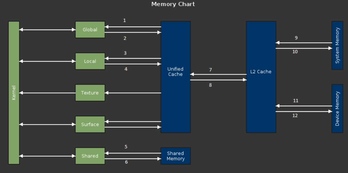
Since we are discussing memory metrics, the following chart shows a GPU memory model with various metrics identified:

-
l1tex__t_sectors_pipe_lsu_mem_global_op_ld.sum,.per_second, l1tex__t_requests_pipe_lsu_mem_global_op_ld.sum
-
l1tex__t_bytes_pipe_lsu_mem_global_op_st.sum, .per_second
-
l1tex__t_sectors_pipe_lsu_mem_local_op_ld.sum, .per_second
-
l1tex__t_sectors_pipe_lsu_mem_local_op_st.sum, .per_second
-
smsp__inst_executed_op_shared_ld.sum, .per_second
-
smsp__inst_executed_op_shared_st.sum, .per_second
-
lts__t_sectors_srcunit_tex_op_read.sum, .per_second
-
lts__t_sectors_srcunit_tex_op_write.sum, .per_second
-
lts__t_sectors_aperture_sysmem_op_read.sum, .per_second
-
lts__t_sectors_aperture_sysmem_op_write.sum, .per_second
-
dram__bytes_read.sum, .per_second
-
dram__bytes_write.sum, .per_second
In the above table, each line corresponds to a numbered path in the diagram. The first entry in each line indicates a cumulative metric (for that path). By appending .per_second to that metric, it can be converted into a throughput metric. For example, dram__bytes_write.sum is a cumulative metric, and dram__bytes_write.sum.per_second is a throughput metric. This table is not an exhaustive list of metrics applicable to each path, but gives some representative examples.
Getting familiar with the Nsight Compute CLI
If you’re familiar with using nvprof, using the Nsight Compute CLI (command line interface) may be the most comfortable. As we’ll see, we can get similar data using either the CLI or the GUI (graphical user interface), but the CLI might be easier if you know specifically what data you are looking for (e.g. running before/after experiments, as we will do here, capturing the same metrics), and/or if you want to use command line style automation (e.g. scripts to compile data). So let’s start there. For this discussion, we will use the linux tool, although windows command line usage should be quite similar (installation paths, and path related characteristics, will be different). One of the first things to know is that the path to the tool may not be set up by default, nor is it part of the /usr/local/cuda/bin path that you may have set up, if you followed the CUDA toolkit install instructions carefully. (In later CUDA toolkits, the path should be setup by default during installation.) The Nsight Compute tool is installed with CUDA toolkit versions 10.0 and later (I strongly recommend using the latest version, at least from CUDA 10.1 Update 1 or later). If you want to or need to, you can install the Nsight Compute tool directly using a standalone installer from https://developer.nvidia.com/nsight-compute. This is also a way to get the latest version. So you’ll either want to add the path to the nsight compute binaries to your PATH environment variable, or else you’ll need to specify the full path when executing it. On CUDA 10.1, the full path is: /usr/local/cuda/NsightCompute-2019.3/, so to fully specify the CLI executable, use: /usr/local/cuda/NsightCompute-2019.3/nv-nsight-cu-cli. At this point you may want to try running the query metrics command from above. For the commands presented in this blog, we will assume that you have added the path to your PATH variable.
While it is not the focus of this blog, there are quite a few capabilities that Nsight Compute offers. We can start by running it in “details page mode” on our executable. Using the code above, compile with nvcc -arch=sm_70 example.cu -o example, modifying the -arch specification to match your GPU. The examples here will use a Volta device (sm_70), but should run equally well on a Turing device. You will not be able to follow this example exactly on an earlier GPU (e.g. Kepler, Maxwell, Pascal) architecture because the available metrics vary between GPUs of compute capability 7.0 and higher, compared to GPUs of compute capability 6.x. Furthermore, use of Nsight Compute is not supported on devices of compute capability 6.0 and lower. To show the details page, try the following:
$ /usr/local/cuda/NsightCompute-2019.3/nv-nsight-cu-cli ./example
==PROF== Connected to process 30244
==PROF== Profiling "matrix_add_2D" - 1: 0%....50%....100% - 48 passes
Success!
==PROF== Disconnected from process 30244
[30244] example@127.0.0.1
  matrix_add_2D, 2019-Jun-06 23:12:59, Context 1, Stream 7
    Section: GPU Speed Of Light
    ----------------------------------------- --------------- ------------------------------
    Memory Frequency                            cycle/usecond                         866.22
    SOL FB                                                  %                          21.46
    Elapsed Cycles                                      cycle                         73,170
    SM Frequency                                cycle/nsecond                           1.21
    Memory [%]                                              %                          56.20
    Duration                                          usecond                          60.16
    SOL L2                                                  %                          53.58
    SOL TEX                                                 %                          60.21
    SM Active Cycles                                    cycle                      68,202.96
    SM [%]                                                  %                           8.97
    ----------------------------------------- --------------- ------------------------------

    Section: Compute Workload Analysis
    ----------------------------------------- --------------- ------------------------------
    Executed Ipc Active                            inst/cycle                           0.18
    Executed Ipc Elapsed                           inst/cycle                           0.17
    Issue Slots Max                                         %                           5.00
    Issued Ipc Active                              inst/cycle                           0.18
    Issue Slots Busy                                        %                           4.57
    SM Busy                                                 %                           9.61
    ----------------------------------------- --------------- ------------------------------

    Section: Memory Workload Analysis
    ----------------------------------------- --------------- ------------------------------
    Memory Throughput                            Gbyte/second                         251.25
    Mem Busy                                                %                          56.20
    Max Bandwidth                                           %                          53.58
    L2 Hit Rate                                             %                          89.99
    Mem Pipes Busy                                          %                           3.36
    L1 Hit Rate                                             %                          90.62
    ----------------------------------------- --------------- ------------------------------

    Section: Scheduler Statistics
    ----------------------------------------- --------------- ------------------------------
    Active Warps Per Scheduler                           warp                          11.87
    Eligible Warps Per Scheduler                         warp                           0.15
    No Eligible                                             %                          95.39
    Instructions Per Active Issue Slot             inst/cycle                              1
    Issued Warp Per Scheduler                                                           0.05
    One or More Eligible                                    %                           4.61
    ----------------------------------------- --------------- ------------------------------

    Section: Warp State Statistics
    ----------------------------------------- --------------- ------------------------------
    Avg. Not Predicated Off Threads Per Warp                                           29.87
    Avg. Active Threads Per Warp                                                          32
    Warp Cycles Per Executed Instruction                cycle                         261.28
    Warp Cycles Per Issued Instruction                                                257.51
    Warp Cycles Per Issue Active                                                      257.51
    ----------------------------------------- --------------- ------------------------------

    Section: Instruction Statistics
    ----------------------------------------- --------------- ------------------------------
    Avg. Executed Instructions Per Scheduler             inst                          3,072
    Executed Instructions                                inst                        983,040
    Avg. Issued Instructions Per Scheduler               inst                       3,116.96
    Issued Instructions                                  inst                        997,428
    ----------------------------------------- --------------- ------------------------------

    Section: Launch Statistics
    ----------------------------------------- --------------- ------------------------------
    Block Size                                                                         1,024
    Grid Size                                                                          1,024
    Registers Per Thread                      register/thread                             16
    Shared Memory Configuration Size                     byte                              0
    Dynamic Shared Memory Per Block                byte/block                              0
    Static Shared Memory Per Block                 byte/block                              0
    Threads                                            thread                      1,048,576
    Waves Per SM                                                                        6.40
    ----------------------------------------- --------------- ------------------------------

    Section: Occupancy
    ----------------------------------------- --------------- ------------------------------
    Block Limit SM                                      block                             32
    Block Limit Registers                               block                              4
    Block Limit Shared Mem                              block                            inf
    Block Limit Warps                                   block                              2
    Achieved Active Warps Per SM                         warp                          48.50
    Achieved Occupancy                                      %                          75.78
    Theoretical Active Warps per SM                warp/cycle                             64
    Theoretical Occupancy                                   %                            100
    ----------------------------------------- --------------- ------------------------------
That’s a lot of output. (If your code has multiple kernel invocations, details page data will be gathered and displayed for each.) We won’t try and go through it all in detail, but notice there are major sections for SOL (speed of light – comparison against best possible behavior), compute analysis, memory analysis, scheduler, warp state, instruction and launch statistics, and occupancy analysis. You can optionally select which of these sections are collected and displayed with command-line parameters. Command-line parameter help is available in the usual way (--help), and also in the documentation. Note the choice of sections and metrics will affect profiling time in general, as well as the size of the output.
We could possibly make some inferences about our objective (global load/store efficiency) using the above data, but let’s focus on the metrics of interest. We gather these in a fashion very similar to how you would do it with nvprof:
$ nv-nsight-cu-cli --metrics l1tex__t_sectors_pipe_lsu_mem_global_op_ld.sum,l1tex__t_requests_pipe_lsu_mem_global_op_ld.sum ./example
==PROF== Connected to process 30749
==PROF== Profiling "matrix_add_2D" - 1: 0%....50%....100% - 4 passes
Success!
==PROF== Disconnected from process 30749
[30749] example@127.0.0.1
  matrix_add_2D, 2019-Jun-06 23:25:45, Context 1, Stream 7
    Section: Command line profiler metrics
    ------------------------------------------------ ------------ ------------------------------
    l1tex__t_requests_pipe_lsu_mem_global_op_ld.sum       request                         65,536
    l1tex__t_sectors_pipe_lsu_mem_global_op_ld.sum         sector                      2,097,152
    ------------------------------------------------ ------------ ------------------------------
This first metric above represents the denominator (requests) of the desired measurement (transactions per request) and the second metric represents the numerator (transactions). If we divide these, we get 32 transactions per request. Therefore, each thread in the warp is generating a separate transaction. This is a good indication that our access pattern (reading, in this case) is not coalesced.
Using the Nsight Compute GUI
What if we wanted to gather these metrics using the GUI? One requirement (for linux), similar to using the NVIDIA Visual Profiler (nvvp) on linux, is that we will need an X session to run the GUI app version in. To get started, from an X-capable session if you were using the Visual Profiler, you would type nvvp at the command prompt. To use Nsight Compute GUI, type:
/usr/local/cuda/NsightCompute-2019.3/nv-nsight-cu
Or just nv-nsight-cu if you already added the path to your PATH variable. Next you should see a window open that looks something like below:

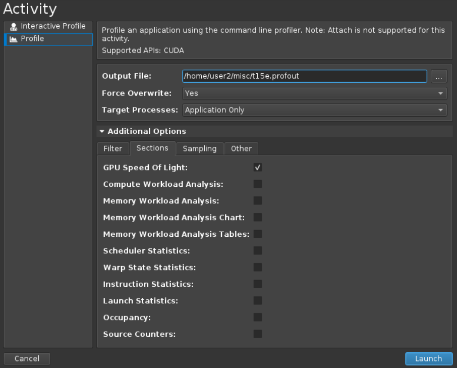
For the easiest start, we can click on Continue under Quick Launch as circled above. (Alternatively, you can create a project by selecting the Create New Project button under New Project.) Next, a profiling configuration window should open (“Connect to process”); you can click on Additional Options at the bottom of the window, then click on the Other tab. We will then enter input on the Application Executable:, Output File:, and Metrics: lines:

Here we entered the path and name of the executable to be profiled (example), the file name where we will store the metric results, and the comma-separated metric names:
l1tex__t_sectors_pipe_lsu_mem_global_op_ld.sum,l1tex__t_requests_pipe_lsu_mem_global_op_ld.sum
After that, you can minimize the Additional Options section and click the blue Launch button. The profiler will then run and capture the requested data, displaying it like this:
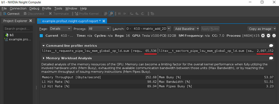
In the picture above, the requested metric data (shown underlined in red above) as well as one other collected section are reported (in this case, Memory Workload Analysis). Note the file saved to disk in this case is not human-readable, but is in a report format designed to be viewed (opened) from the Nsight Compute GUI. For a human-readable file copy, most pages in the report have export buttons available, usually in the upper-right corner.
If you want to explore GUI features in more detail, the documentation contains a quick-start section introducing the GUI.
Fixing the Code
The reason for the low-efficiency (high number of transactions per request) in this code is due to our method of 2D indexing:
... C[idx][idy] = A[idx][idy] + B[idx][idy];
The index built with threadIdx.x (i.e. idx) should appear in the last subscript for coalesced access across a warp; instead, it appears in the first subscript. While either method can give correct results, they are not the same from a performance perspective. This arrangement results in each thread in a warp accessing data in a “column” in memory, rather than a “row” (i.e. adjacent). We can fix this by modifying our kernel code as follows:
__global__ void matrix_add_2D(const arr_t * __restrict__ A, const arr_t * __restrict__ B, arr_t * __restrict__ C, const size_t sw, const size_t sh){

  size_t idx = threadIdx.x+blockDim.x*(size_t)blockIdx.x;
  size_t idy = threadIdx.y+blockDim.y*(size_t)blockIdx.y;

  if ((idy < sh) && (idx < sw)) C[idy][idx] = A[idy][idx] + B[idy][idx];
}
The only change is to the last line of code, where we reversed the usage of idx and idy. When we recompile and run the same profiling experiment on this modified code, we see:
$ nv-nsight-cu-cli --metrics l1tex__t_sectors_pipe_lsu_mem_global_op_ld.sum,l1tex__t_requests_pipe_lsu_mem_global_op_ld.sum ./example
==PROF== Connected to process 5779
==PROF== Profiling "matrix_add_2D" - 1: 0%....50%....100% - 4 passes
Success!
==PROF== Disconnected from process 5779
[5779] example@127.0.0.1
  matrix_add_2D, 2019-Jun-11 12:01:26, Context 1, Stream 7
    Section: Command line profiler metrics
    ----------------------------------------------- --------------- ------------
    l1tex__t_requests_pipe_lsu_mem_global_op_ld.sum         request       65,536
    l1tex__t_sectors_pipe_lsu_mem_global_op_ld.sum           sector      262,144
    ----------------------------------------------- --------------- ------------
Now the ratio of the metrics is 4:1 (transactions per request), indicating the desired transaction size of 32 bytes is achieved, and the efficiency of loads (and stores) is substantially improved over the previous case.
Since this work involves a comparison of a new result to an older (comparable) result, we can demonstrate an additional feature of the GUI. We can use the GUI to collect profiling results for both cases, and show the comparison. We collect the first set of results as described above. Leave the GUI open. Then select the Connect button in the upper-left corner of the GUI, and simply change the output file to a new name. If needed, you should also change the file name to be profiled to the modified version. After doing this, the blue Launch button is available again. Press the Launch button to create a New Results tab with the data from the new, modified code run. Finally, select the Original Results tab, then press the Add Baseline button at the top. Then select the New Results tab, and any differences in metrics are reported:
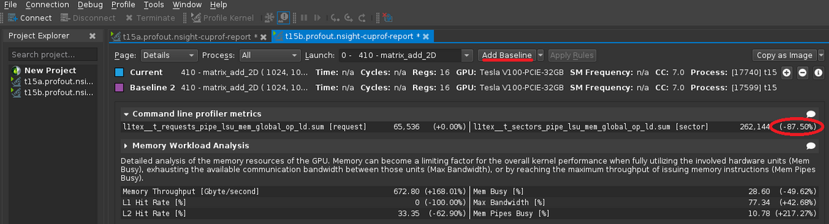
In the above case, we see the improved metric is shown as an 87.5% reduction compared to the baseline (an 8:1 reduction in transactions).
So does this help? The reason we are interested in making this change is because improving the memory usage efficiency should improve the performance of this memory-bound code. That means things should run faster. In order to verify that, we can use the Nsight Systems profiler covered in the previous blog to check the kernel duration before, and after the change. In order to do this, we could use the Nsight Systems CLI, and use a command similar to the first CLI command presented in the previous blog (requires Nsight Systems version 2019.3.6 or newer):
$ nsys profile -o example.nsysprofout --stats=true ./example
However, since the focus of this blog is on Nsight Compute, we could make a similar measurement using the Elapsed Cycles data from the GPU SOL report section. We can also use the comparison method outlined in the last section. In the GUI, we can start by selecting the Connect button in the upper left hand corner, to open the profiling configuration settings. Select the Additional Options drop-down again, and you can clear out the metrics from the Other tab. Now select the Sections tab, and select the GPU Speed of Light section (and you can deselect all other sections, to simplify the output and reduce profiling time). You may also need to change the output file name for this new profiling session. The blue Launch button should then appear.
Click the Launch button to collect the new profiling data. As in the previous activity, we will repeat these steps for the original version of the application and also for the improved version. After that, we can then set the original version as a baseline, and see the improvement in the elapsed cycles SOL output:

Based on the above data, we see the change resulted in about a 68% reduction in kernel execution duration (elapsed cycles).
Careful study of the other data contained in the Memory Analysis sections of the Nsight Compute output (whether in the GUI or CLI output) will also show the beneficial effect of this change on other analysis data.
What Else is New?
There are many new features in Nsight Compute compared to the NVIDIA Visual Profiler and nvprof, and we’ve only touched on a few in this blog.
New features in Nsight Compute GUI compared to Visual Profiler:
- Comparing profile results within the tool
- Interactive profiling mode (with API stream and parameter capture)
- Remote launch/attach with cross-OS support
New features in Nsight Compute GUI and CLI compared to Visual Profiler/nvprof:
- More detailed metric coverage
- Customizable metric sections and python-based guided analysis
- More stable data collection (clock control, cache resets, …)
- Reduced overhead for kernel replay (diff after first pass)
- Support for new CUDA/NVTX features (e.g. graphs support, nvtx filter descriptions)
Conclusion
The new tools are intended to provide the same (and better) capability compared to nvprof and the Visual Profiler, but will require some new setup and new methods to get similar results. With respect to metrics profiling which is the primary focus of this blog, it’s important to become familiar with the new metrics, and if need be, synthesize the data you are looking for, from combinations of these metrics. For users transitioning from nvprof, the Transition Guide in the documentation for Nsight Compute will be especially helpful. Looking for more help or have additional questions? Visit the NVIDIA Developer forums and browse or ask a question in the Nsight Compute forum.